3.2 Transfer Functions
In this section, the nonrecursive digital filter
$$ f_n = \sum_{k=-K}^K c_k\,y_{n-k} \tag{NF} $$is investigated, where $\,K\,$ is a positive integer, and the filter coefficients $\,c_k\,$ are real numbers.
Under certain symmetry requirements on the coefficients $\,c_k\,,$ the action of this filter on sums of sinusoidal components is easily explained, via the transfer function corresponding to the filter. The development of the transfer function calls on the linear algebra concepts of eigenvalues and eigenvectors, so a quick review is in order:
Vector spaces and linear transformations between vector spaces are reviewed in Appendix $2$. The definitions of eigenvalue and eigenvector are given next.
Let $\,V\,$ be a vector space over $\,\Bbb F\,,$ and let $\,T\,$ be a linear transformation from $\,V\,$ into $\,V\,.$
An eigenvalue of $\,T\,$ is a scalar $\,\lambda\in\Bbb F\,$ for which there exists a nonzero vector $\,v\in V\,$ with $\,Tv = \lambda v\,.$
If $\,\lambda\,$ is an eigenvalue of $\,T\,,$ then any nonzero vector $\,v\,$ satisfying $\,Tv = \lambda v\,$ is called an eigenvector of $\,T\,$ corresponding to $\,\lambda\,.$
It is important to observe that the action of $\,T\,$ on its eigenvectors is particularly simple—it is just scalar multiplication. That is, the linear transformation $\,T\,$ maps an eigenvector $\,v\,$ to the scaled vector $\,\lambda v\,.$ Note also that any eigenvalue of a linear transformation between real vector spaces is, by definition, a real number.
Let $\,\Bbb R^\infty\,$ denote the set of ‘doubly infinite’ lists with a designated origin; i.e., each member of $\,\Bbb R^\infty\,$ is of the form
$$ (\ldots,y_{-3},y_{-2},y_{-1},\widehat{y_0},y_1,y_2,y_3,\ldots)\ , $$where $\,y_i\in\Bbb R\,$ for all integers $\,i\,,$ and the element indicated by the ‘$\,\widehat{\hphantom{x}}\,$’ is the origin. The ‘origin’ is needed for a well-defined addition on $\,\Bbb R^\infty\,,$ and will only be shown when necessary.
For an element of $\,\Bbb R^\infty\,,$ define multiplication by $\,\alpha\in\Bbb R\,$ via:
$$ \begin{align} &\alpha(\ldots,y_{-1},\widehat{y_0},y_1,\ldots)\cr\cr &\quad := (\ldots,\alpha y_{-1},\widehat{\alpha y_0},\alpha y_1,\ldots) \end{align} $$Addition in $\,\Bbb R^\infty\,$ is defined by first aligning the origins of the elements being added, and then adding componentwise:
$$ \begin{alignat}{5} &(\ldots,& x_{-1}&,& \widehat{x_0}&,& x_1&,& \ldots &)\cr\cr +\ &(\ldots,& y_{-1}&,& \widehat{y_0}&,& y_1&,& \ldots &)\cr\cr =\ &(\ldots,&\ \ x_{-1} + y_{-1}&,&\ \ \widehat{x_0 + y_0}&,&\ \ x_1 + y_1&,&\ \ \ldots &) \end{alignat} $$With this addition and multiplication by real numbers, $\,\Bbb R^\infty\,$ is a real vector space.
In preparation for viewing the nonrecursive filter (NF) as a linear transformation between vector spaces, it is first necessary to view finite input lists $\,(y_n)\,$ and output lists $\,(f_n)\,$ as elements of $\,\Bbb R^\infty\,.$
Every finite list $\,(y_n)_{n=1}^N\,$ of data values can be associated with an element of $\,\Bbb R^\infty\,$ by ‘padding it with zeros’ in both directions, and designating $\,y_1\,$ as the origin; that is:
$$ \begin{align} &(y_1,y_2,\ldots,y_N)\cr &\quad \mapsto (\ldots,0,0,0,\widehat{y_1},y_2,\ldots,y_N,0,0,0,\ldots) \end{align} $$Once this association with an element in $\,\Bbb R^\infty\,$ is made, there is no longer a ‘filter lag’ problem: that is, filtered values $\,f_i\,$ can be found for all integers $\,i\,.$ In this way, one has the following input and output lists in $\,\Bbb R^\infty\,$:
$$ \begin{alignat}{11} &(&\ldots\, &,& 0 &,& 0 &,& \widehat{y_1} &,& y_2 &,&\ldots\, &,& y_N &,& 0 &,& 0 &,& \ldots &)\cr\cr &(&\ldots\, &,&\ \ f_{-1} &,&\ \ f_0 &,&\ \ \widehat{f_1} &,&\ \ f_2 &,&\ \ \ldots\, &,&\ \ f_N &,&\ \ f_{N+1} &,&\ \ f_{N+2} &,&\ \ \ldots &) \end{alignat} $$Note that $\,f_n\,$ will be zero, for values of $\,n\,$ that are sufficiently large, and sufficiently negative.
Next, the nonrecursive filter (NF) is used to define a transformation from $\,\Bbb R^\infty\,$ to $\,\Bbb R^\infty\,,$ and it is shown that this transformation is linear. In the following discussion, it is assumed that the (finite) list $\,(y_n)_{n=1}^N\,$ and the filter list $\,(f_n)\,$ are associated with elements in $\,\Bbb R^\infty\,,$ as discussed above.
Let $\,F : \Bbb R^\infty \to \Bbb R^\infty\,$ be defined by $\,F({\bf y}) := {\bf f}\,,$ where $\,{\bf y} := (y_n)\,$ is a list of data values, and $\,{\bf f} := (f_n)\,$ is its corresponding list of filter values, with:
$$ f_n = \sum_{k=-K}^K c_k\,y_{n-k} \tag{1} $$For the remainder of this section, the entry $\,f_n\,$ of $\,F({\bf y})\,$ is optionally denoted by $\,F({\bf y})_n\,,$ the entry $\,y_n\,$ of $\,{\bf y}\,$ by $\,{\bf y}_n\,,$ and the sum $\,\sum_{k=-K}^K\,$ by $\,\sum_k\,.$ With this notation, the sum in ($1$) is rewritten as:
$$ F({\bf y})_n = \sum_{k} c_k\,{\bf y}_{n-k} $$Let $\,{\bf x} = (x_n)_{n=-\infty}^\infty\,$ and $\,{\bf y} = (y_n)_{n=-\infty}^\infty\,$ be elements of $\,\Bbb R^\infty\,.$ Then,
$$ \begin{align} F({\bf x} + {\bf y})_n &= \sum_k c_k({\bf x} + {\bf y})_{n-k}\cr\cr &= \sum_k c_k\,{\bf x}_{n-k} + \sum_k c_k\,{\bf y}_{n-k}\cr\cr &= F({\bf x})_n + F({\bf y})_n\ , \end{align} $$which implies that $\,F({\bf x} + {\bf y}) = F({\bf x}) + F({\bf y})\,.$ Also, for $\,\alpha\in\Bbb R\,,$
$$ \begin{align} F(\alpha{\bf x})_n &= \sum_k c_k(\alpha {\bf x})_{n-k}\cr\cr &= \alpha\sum_k c_k\,{\bf x}_{n-k}\cr\cr &= \alpha F({\bf x})_n\ , \end{align} $$which implies that $\,F(\alpha {\bf x}) = \alpha F({\bf x})\,.$ Thus, $\,F\,$ is a linear operator from $\,\Bbb R^\infty\,$ to $\,\Bbb R^\infty\,.$
Let $\,\Delta T\,$ be a positive real number, and let $\,\omega\in\Bbb R\,.$
As a motivation for later results, define a list $\,{\bf e}_\omega\,$ via:
$$ ({\bf e}_\omega)_n := e^{i\omega n\Delta T} $$The sketch below illustrates some list entries when $\,\omega \gt 0\,.$
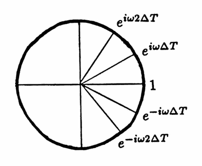
Use $\,{\bf e}_\omega\,$ as the input list to the nonrecursive filter (NF). In so doing, one obtains the output list $\,(f_n)\,,$ where
$$ \begin{align} f_n &= \sum_k c_k({\bf e}_\omega)_{n-k}\cr\cr &= \sum_k c_k e^{i\omega(n-k)\Delta T}\cr\cr &= \sum_k c_ke^{i\omega n\Delta T}e^{-i\omega k\Delta T}\cr\cr &= \left( \sum_k c_k e^{-i\omega k\Delta T} \right)e^{i\omega n\Delta T}\cr\cr &:= C\cdot ({\bf e}_\omega)_n\ , \end{align} $$where $\,C := \sum_{k=-K}^K c_k e^{-i\omega k\Delta T}\,.$ Thus, when the list $\,{\bf e}_\omega\,$ is input to (NF), the filtered list $\,C{\bf e}_\omega\,$ emerges. In general, $\,C\,$ may not be a real number. However, the next result shows that under certain symmetry requirements on the filter coefficients $\,c_k\,,$ $\,C\,$ will be real:
Let $\,c_k\,,$ $\,-K\le k\le K\,,$ be real numbers satisfying:
$$ c_k = c_{-k}\ \ \text{for}\ \ k = 1,\ldots,K $$Then, the number
$$ C := \sum_{k=-K}^K c_k e^{-i\omega k\Delta T} $$is real, for all real numbers $\,\omega\,$ and $\,\Delta T\,.$
Proof
$$ \begin{align} &\sum_{k=-K}^K c_ke^{-i\omega k\Delta T}\cr\cr &\quad = c_0 + \sum_{k=1}^K c_ke^{-i\omega k\Delta T} + \sum_{k=-1}^{-K} c_k e^{-i\omega k\Delta T}\cr\cr &\quad = c_0 + \sum_{k=1}^K c_ke^{-i\omega k\Delta T} + \overbrace{\sum_{j=1}^K c_{-j}e^{i\omega j\Delta T}}^{j := -k}\cr\cr &\quad = c_0 + \sum_{k=1}^K c_ke^{-i\omega k\Delta T} + \sum_{j=1}^K c_j e^{i\omega j\Delta T}\cr\cr &\quad = c_0 + \sum_{k=1}^K c_k(e^{-i\omega k\Delta T} + e^{i\omega k\Delta T})\cr\cr &\quad = c_0 + \sum_{k=1}^K c_k\bigl( 2\cos(\omega k\Delta T) \bigr)\ , \end{align} $$which is a real number. $\blacksquare$
A nonrecursive digital filter
$$ f_n = \sum_{k=-K}^K c_k\,y_{n-k} $$for which $\,c_k = c_{-k}\,,$ $k = 1,\ldots,K\,,$ is called symmetric.
The next result shows that any nonzero list in $\,\Bbb R^\infty\,$ that is formed by evaluating the functions $\,\sin(\omega t)\,$ and $\,\cos(\omega t)\,$ at the time values
$$ \begin{gather} (\ldots\,,\,t_1 - 2\Delta T\,,\, t_1 - \Delta T\,,\,\cr \widehat{t_1}\,,\,\cr t_1 + \Delta T\,,\,t_1 + 2\Delta T\,,\,\ldots)\ , \end{gather} $$where $\,t_1\in\Bbb R\,,$ $\,\Delta T \gt 0\,,$ and $\,\omega\in\Bbb R\,,$ is an eigenvector for the linear transformation $\,F\,:\,\Bbb R^\infty\to\Bbb R^\infty\,$ defined in ($1$), providing that the nonrecursive filter used to define $\,F\,$ is symmetric:
Let $\,t_1\in\Bbb R\,,$ $\,\Delta T\gt 0\,,$ and $\,\omega\in\Bbb R\,.$ Form lists
$$ \begin{gather} \bigl( \sin\omega(t_1 + n\Delta T) \bigr)_{n=-\infty}^\infty\cr \text{and}\cr \bigl( \cos\omega(t_1 + n\Delta T) \bigr)_{n=-\infty}^\infty \end{gather} \tag{2} $$in $\,\Bbb R^\infty\,$ by evaluating the functions $\,\sin \omega t\,$ and $\,\cos\omega t\,$ on the time list:
$$ \begin{gather} (\ldots,t_1 - 2\Delta T, t_1 - \Delta T,\cr \widehat{t_1},\cr t_1 + \Delta T,t_1 + 2\Delta T,\ldots) \end{gather} $$Assume that $\,t_1\,,$ $\,\Delta T\,$ and $\,\omega\,$ are such that the lists in ($2$) are nonzero.
Then, the lists in ($2$) are eigenvectors for the linear transformation $\,F\,:\,\Bbb R^\infty\to\Bbb R^\infty\,$ defined by the symmetric nonrecursive filter:
$$ \begin{gather} f_n = \sum_{k=-K}^K c_k\,y_{n-k}\ ,\cr\cr c_k = c_{-k}\ \ \text{for}\ \ k = 1,\ldots,K \end{gather} $$Both lists have corresponding eigenvalue:
$$ \sum_{k=-K}^K c_k e^{-i\omega k\Delta T} $$Proof
The following argument uses the facts that for all $\,z\,, w\in\Bbb C\,$ and for all $\,\alpha\,, \beta\in\Bbb R\,,$
$$ \begin{gather} \text{Re}(\alpha z + \beta w) = \alpha\,\text{Re}(z) + \beta\,\text{Re}(w)\cr\cr \text{Im}(\alpha z + \beta w) = \alpha\,\text{Im}(z) + \beta\,\text{Im}(w) \end{gather} $$where $\,\text{Re}(z)\,$ and $\,\text{Im}(z)\,$ denote the real and imaginary parts, respectively, of a complex number $\,z\,.$
Define
$$ C := \sum_{k=-K}^K c_k\, e^{-i\omega k\Delta T}\ , $$and recall that $\,C\,$ is a real number, since $\,c_k = c_{-k}\,$ for $\,k = 1,\ldots,K\,.$ Also define
$$ {\bf S} := \bigl( \sin \omega(t_1 + n\Delta T) \bigr)_{n=-\infty}^\infty\ , $$so that:
$$ {\bf S}_n = \sin\omega(t_1 + n\Delta T) $$Then:
$$ \begin{align} F({\bf S})_n &= \sum_k c_k\,\sin\omega\bigl( t_1 + (n-k)\Delta T \bigr)\cr\cr &= \sum_k c_k\,\text{Im} \bigl( e^{i\omega(t_1 + (n-k)\Delta T)} \bigr)\cr\cr &= \text{Im} \left( \sum_k c_k\,e^{i\omega(t_1 + (n-k)\Delta T)} \right)\cr\cr &= \text{Im} \left( \sum_k c_k\,e^{i\omega(t_1 + n\Delta T)}e^{-i\omega k\Delta T} \right)\cr\cr &= \text{Im} \left( e^{i\omega(t_1 + n\Delta T)} \overbrace{\sum_k c_k\,e^{-i\omega k\Delta T}}^{\text{real number}} \right)\cr\cr &= C\cdot \text{Im} \bigl( e^{i\omega(t_1 + n\Delta T)} \bigr)\cr\cr &= C\cdot \bigl( \sin\omega(t_1 + n\Delta T) \bigr)\cr\cr &= C\cdot {\bf S}_n \end{align} $$It follows that $\,F({\bf S}) = C{\bf S}\,.$ Thus, $\,{\bf S}\,$ is an eigenvector for $\,F\,$ with eigenvalue $\,C\,.$
By defining
$$ {\bf C} := \bigl( \cos\omega(t_1 + n\Delta T) \bigr)_{n=-\infty}^\infty\ , $$and replacing $\,{\bf S}\,$ by $\,{\bf C}\,,$ $\,\sin\,$ by $\,\cos\,,$ and $\,\text{Im}\,$ by $\,\text{Re}\,$ in the argument above, it follows that $\,{\bf C}\,$ is also an eigenvector for $\,F\,$ with eigenvalue $\,C\,.$ $\blacksquare$
Let $\,F\,$ be the symmetric nonrecursive filter given by:
$$ \begin{gather} f_n = \sum_{k=-K}^K c_k\,y_{n-k}\ ,\cr\cr c_k = c_{-k}\ \ \text{for}\ \ k = 1,\ldots,K \end{gather} $$Let $\,\Delta T\,$ be a fixed positive number. The function $\, H\,:\,\Bbb R\to\Bbb R\,$ defined by
$$ \begin{align} H(\omega) &:=\sum_{k=-K}^K c_k\,e^{-i\omega k\Delta T}\cr\cr &= c_0 + \sum_{k=1}^K 2c_k\cos(\omega k\Delta T) \end{align} $$is called the transfer function corresponding to $\,F\,$ and spacing $\,\Delta T\,$ .
The transfer function has the property that when the functions $\,\sin\omega t\,$ or $\,\cos\omega t\,$ are sampled at the equally-spaced time values
$$ \begin{gather} (\ldots\,,\,t_1-2\Delta t\,,\,t_1-\Delta T\,,\,\cr t_1\,,\cr t_1 + \Delta T\,,\,t_1 + 2\Delta T\,,\,\dots)\ , \end{gather} $$and then input to the symmetric nonrecursive filter, the same lists emerge, except scaled by the constant $\,H(\omega)\,.$
Since $\,F\,$ is linear, if a sum of sinusoidal components is input to $\,F\,,$ then the same sum will emerge, with each component appropriately scaled. The examples following the next lemma illustrate this process.
Proof
$$ \begin{align} &H\bigl( \omega + \frac{2\pi}{\Delta T} \bigr)\cr\cr &\quad = \sum_{k=-K}^K c_k\,e^{-i(\omega+\frac{2\pi}{\Delta T})k\Delta T}\cr\cr &\quad = \sum_{k=-K}^K c_k\,e^{-i\omega k\Delta T} \overbrace{e^{-i2\pi k}}^{= 1}\cr\cr &\quad = H(\omega)\ \ \ \blacksquare \end{align} $$Thus, it suffices to study the transfer function $\,H\,$ on any interval of length $\,\frac{2\pi}{\Delta T}\,,$ say the interval $\,[0,\frac{2\pi}{\Delta T}]\,.$
Let $\,K \ge 3\,$ be an odd integer. Let $\,K = 2m + 1\,$ for a positive integer $\,m\,.$ The smoothing by $K$’s filter,
$$ f_n = \frac 1K\sum_{k=-m}^m y_{n-k}\ , $$has coefficients:
$$ c_{-m} = \cdots = c_{-1} = c_0 = c_1 = \cdots = c_m = \frac 1K $$The corresponding transfer function is:
$$ \begin{align} H(\omega) &= c_0 + \sum_{k=1}^m 2c_k\,\cos(\omega k\Delta T)\cr\cr &= \frac 1K\left( 1 + 2\sum_{k=1}^m \cos(\omega k\Delta T) \right) \end{align} $$The positive number $\,\omega\,$ gives the radian frequency of the functions $\,\sin\omega t\,$ and $\,\cos\omega t\,.$ It is usually more convenient to work with the transfer function expressed in terms of cyclic frequency $\,f\,,$ where $\,\omega = 2\pi f\,.$ To this end, define a function $\,\tilde{H}\,$ by:
$$ \tilde H(f) := H(2\pi f) = H(\omega) $$Therefore:
$$ \begin{align} \tilde H(f) &= \sum_{k=-K}^K c_k e^{-i2\pi f k \Delta T}\cr\cr &= c_0 + \sum_{k=1}^K 2c_k\cos(2\pi f k \Delta T) \end{align} $$Since $\,H\,$ has period $\,\frac{2\pi}{\Delta T}\,,$ it follows that $\,\tilde H\,$ has period $\,\frac 1{\Delta T}\,$:
$$ \begin{align} \tilde H\bigl( f + \frac 1{\Delta T} \bigr) &:= H\bigl( 2\pi(f + \frac 1{\Delta T}) \bigr)\cr\cr &= H\bigl( 2\pi f + \frac{2\pi}{\Delta T} \bigr)\cr\cr &= H(2\pi f)\cr\cr &:= \tilde H(f) \end{align} $$With a sample spacing of $\,\Delta T\,,$ it is unreasonable to try and detect periods less than $\,2\Delta T\,,$ since these smaller periods are ‘confused’ with larger ones due to the effects of aliasing (see these earlier pages and the sketch below). For this reason, the function $\,\tilde H\,$ is only graphed, in practice, on the interval of cyclic frequencies $\,[0,\frac 1{2\Delta T}]\,.$
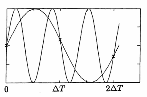
Only periods greater than $\,2\Delta T\,$ can be detected
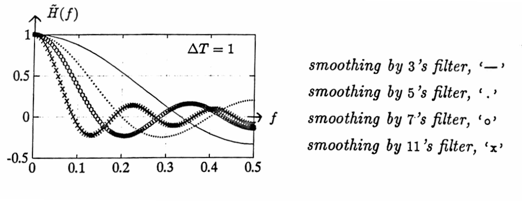
The functions $\,\tilde H\,$ corresponding to the smoothing by $K$’s filters are graphed next, for various values of $\,K\,$ and $\,\Delta T\,.$
The graph below illustrates why the smoothing by $K$’s filters are commonly referred to as low-pass filters: they tend to pass low frequencies ($\,\tilde H(f)\,$ is close to $\,1\,$) and suppress high frequencies ($\,\tilde H(f)\,$ is close to $\,0\,$).
The graph below illustrates that a smaller sampling time $\,\Delta T\,$ allows detection of higher frequencies (smaller periods). For example, the function $\,\tilde H\,$ corresponding to $\,\Delta T = 0.2\,$ gives information about frequencies in the interval $\,[0,2.5]\,,$ whereas when $\,\Delta T = 1\,,$ information is only obtained on the interval $\,[0,0.5]\,.$

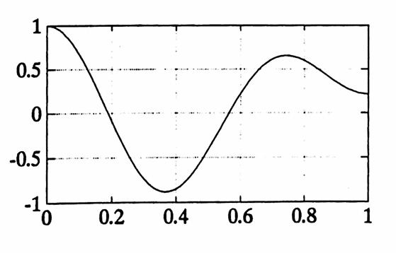
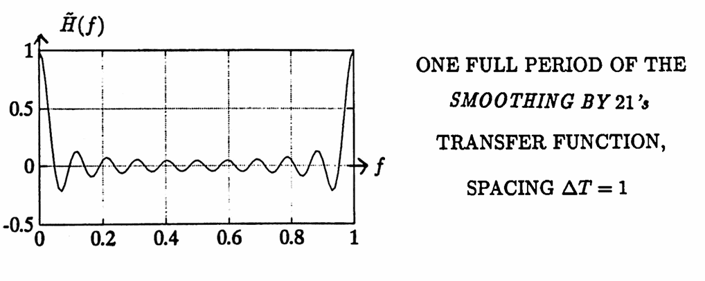
When $\,K\,$ is large, the smoothing by $K$’s filter does a better job of erasing high frequencies. For example, the graph below shows one full period of the transfer function corresponding to the smoothing by $21$’s filter, with sample spacing $\,\Delta T = 1\,.$
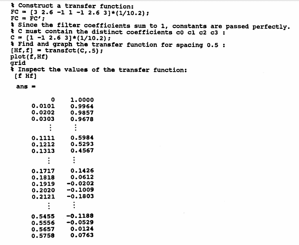
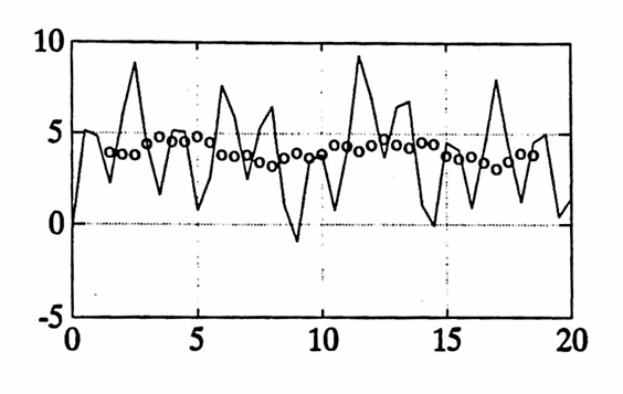
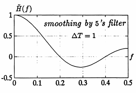
The transfer function for the smoothing by $5$’s filter, $\,\Delta T = 1\,,$ is graphed below. Observe that $\,\tilde H(0.2) = 0\,,$ and $\,\tilde H(0.1) \approx 0.65\,.$
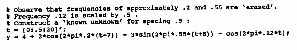
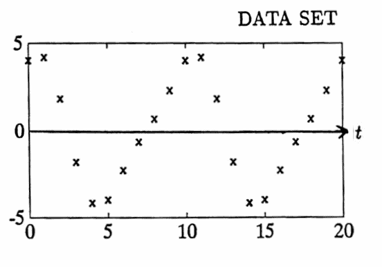
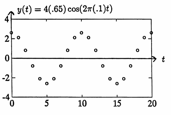
Construct a list $\,(y_n)\,$ by evaluating the function
$$ f(t) = \sin\bigl(2\pi(0.2)t\bigr) + 4\cos\bigl(2\pi(0.1)t\bigr) $$at each number in the uniform time list $\,(\Delta T = 1\,$):
$$ (0,1,2,\ldots,20) $$The function $\,f\,$ has a component of cyclic frequency $\,0.2\,$ (period $\,5\,$), amplitude $\,1\,$; and a component of cyclic frequency $\,0.1\,$ (period $\,10\,$), amplitude $\,4\,.$
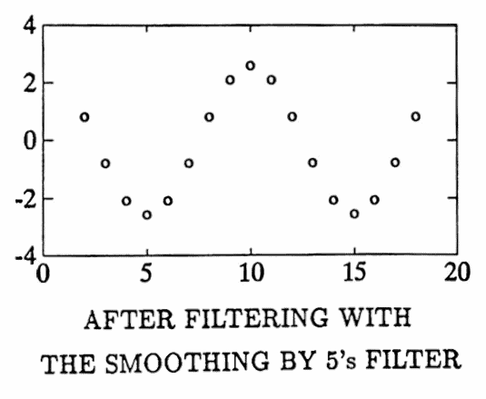
When the list $\,(y_n)\,$ is input to the smoothing by $5$’s filter, the period-$5$ component should emerge, scaled by $\,\tilde H(0.2) = 0\,$; that is, it should be completely erased.
The period-$10$ component should emerge, scaled by $\,\tilde H(0.1) \approx 0.65\,$; thus, its new amplitude should be approximately $\,(0.65)(4) = 2.6\,.$
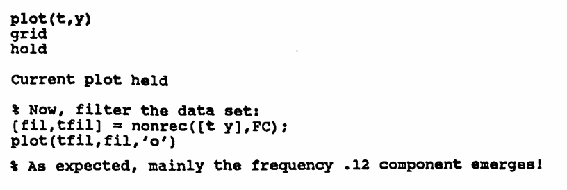
The graphs below illustrate that the filter behaves as dictated by its transfer function.
As a second example, the transfer function for the smoothing by $11$’s filter, with $\,\Delta T = 0.2\,,$ is graphed below. Observe that $\,\tilde H(0.2) \approx 0.7\,.$
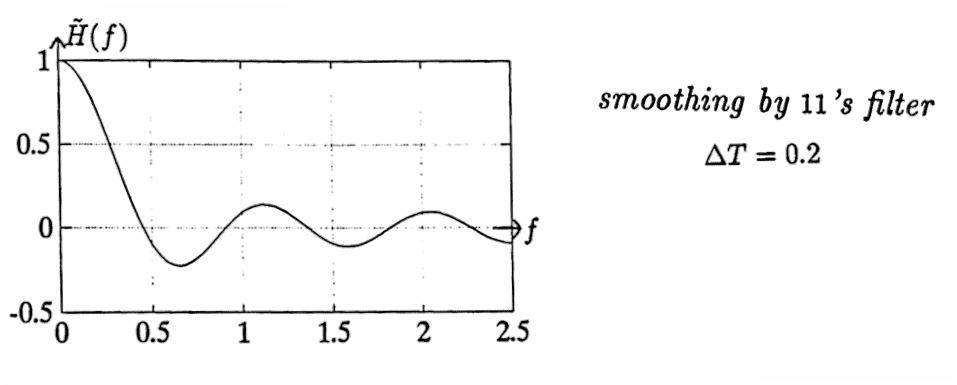
Construct a list $\,(y_n)\,$ by evaluating the function
$$ f(t) = \sin\bigl( 2\pi(0.2)t\bigr) $$at each number in the uniform time list ($\,\Delta T = 0.2\,$):
$$ (0,0.2,0.4,\ldots,20) $$The function $\,f\,$ has cyclic frequency $\,0.2\,$ (period $\,5\,$), and amplitude $\,1\,.$
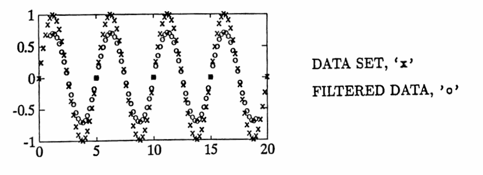
When the list $\,(y_n)\,$ is input to the smoothing by $11$’s filter, it should emerge, scaled by $\,\tilde H(0.2) \approx 0.7\,.$
The graph below illustrates that the filter behaves as dictated by its transfer function.
A MATLAB program for finding the transfer function corresponding to a symmetric nonrecursive filter, and spacing $\,\Delta T\,,$ is given next.
MATLAB Implementation: Finding the Transfer Function for a Symmetric Nonrecursive Filter
transfct(C,dT)
The MATLAB function transfct, with source code given below, computes the transfer function $\,\tilde H\,$ corresponding to a symmetric nonrecursive filter
$$ \begin{gather} f_n = \sum_{k=-K}^K c_k\,y_{n-k}\,,\cr\cr c_k = c_{-k}\ \ \text{for}\ \ k = 1,\ldots,K\,, \end{gather} $$
and spacing $\,\Delta T\,.$
To use the function, type:
[Hf,f] = transfct(C,dT);
The transfer function is then plotted with the command:
plot(f, Hf)
The function requires the following inputs:
-
The $\,K+1\,$ distinct filter coefficients:
$$ c_0,c_1,\ldots,c_K $$These must be stored in the (row or column) vector C .
- The spacing $\,\Delta T\,,$ where $\,\Delta T \gt 0\,$; this is given by the MATLAB variable dT .
The program outputs two column vectors, Hf and f .
The vector f contains $\,100\,$ equally-spaced values from the interval $\,[0,\frac{1}{2\Delta T}]\,.$
The vector Hf contains the values $\,\tilde H($f$)\,.$
The source code for the function transfct is given next:
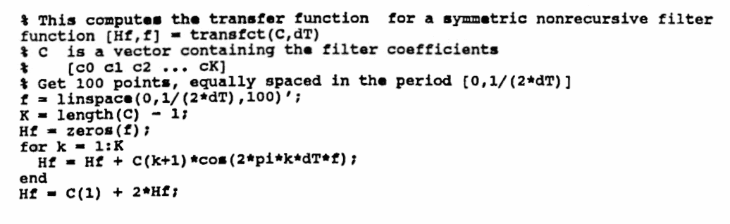
- zeros(size(f))
- endfunction as the last line
The following diary of an actual MATLAB session illustrates the use of transfct . The function nonrec , for applying a non-recursive filter, was discussed in Section $3.1$.