Chapter 3: Filter Theory

3.1 Mathematical Filters

What is a mathematical filter?

A (non-mathematical) ‘filter’ is usually a mechanical device used to process material, often to extract a particular component, like only the finest particles in a granular sand mixture.

A mathematical filter is used for a similar purpose—to process data in some desirable way. For example, filters are used for removal of noise, smoothing, separation of signals, differentiating, and integrating.

Analog versus digital filters

Analog filters are used to process continuous signals, and digital filters are used to process discrete signals that are equally-spaced; that is, data sets $\,\{(t_i,y_i)\}_{i=1}^N\,$ where the time list is uniform.

Notation for digital filters

Let $\,(y_n)\,$ be a list of data values that arose from a data set with a uniform time list. The list $\,(y_n)\,$ is assumed to be of the form $\,(y_n)_{n=1}^N\,$ or $\,(y_n)_{n=-\infty}^\infty\,.$

A digital filter is a function that acts on the list $\,(y_n)\,,$ and produces a new ‘filtered’ list, $\,(f_n)\,,$ where

$$ f_n = \sum_{k=-\infty}^\infty c_ky_{n-k} + \sum_{k=-\infty}^\infty d_k f_{n-k}\ , $$

and where $\,c_k\,$ and $\,d_k\,$ are real constants. For finite lists $\,(y_n)_{n=1}^N\,,$ $\,f_n\,$ is defined if and only if:

$$ 1\le n-k \le N\ \ \text{whenever}\ \ c_k\ne 0 $$

Filter coefficients

The numbers $\,c_k\,$ and $\,d_k\,$ are called the filter coefficients. In practice, all but a finite number of the filter coefficients are zero, so that the sums are actually finite.

Expression is ‘centered’ at $\,y_n$

The subscripts $\,n - k\,$ serve to ‘center’ the expression at $\,y_n\,,$ as illustrated below. In the following diagram, all coefficients $\,d_k\,$ are assumed to be zero.

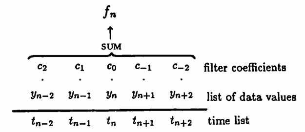
subscripts n-k center the expression at y_n

The data point $\,(t_n,y_n)\,$ corresponds to the filter point $\,(t_n,f_n)\,.$

Current, past, and future values

When filter value $\,f_n\,$ is being computed, $\,f_n\,$ is called the current filter value, and $\,y_n\,$ is called the current data value. The numbers $\,f_{n-k}\,$ and $\,y_{n-k}\,,$ for $\,k = 1,\ldots,\infty\,,$ are called the past filter and data values, respectively. The numbers $\,f_{n-k}\,$ and $\,y_{n-k}\,,$ for $\,k = -1,\ldots,-\infty\,,$ are called the future filter and data values, respectively.

Nonrecursive filters, all $\,d_k = 0\,$

If all coefficients $\,d_k\,$ are zero, then only the data values $\,y_n\,$ are used to compute the filter output. In this case, the filter is called nonrecursive.

Recursive filters, some $\,d_k\ne 0\,$

If any of the coefficients $\,d_k\,$ are nonzero, then computation of $\,f_n\,$ requires other filter values. In this case, the filter is called recursive. In particular, if future values of the filter are used, then a system of linear algebraic equations must be solved to find $\,f_n\,.$

Primarily nonrecursive digital filters will be discussed in this dissertation.

Example: Trapezoid Rule for Approximate Integration is a Recursive Filter

Let $\,\{(t_i,y_i)\}_{i=1}^N\,$ be a data set with a uniform time list having spacing $\,\Delta T \gt 0\,.$ If this data set arose by sampling from a continuous function $\,f\,,$ that is, if $\,y_n = f(t_n)\,,$ then one may wish to use these values to approximate the integral:

$$ \int_{t_1}^{t_n} f(t)\,dt\,,\ \ \text{for}\ n = 2,\ldots,N \tag{1} $$ Recursive filter example: the trapezoid rule for integration

Let $\,f_n\,$ be the approximation to ($1$) that is obtained by using the Trapezoid Rule for approximation (e.g., see [S&B, p.121]). Set $\,f_1 := 0\,.$ Then:

$$ \begin{gather} f_n = \frac 12\Delta T(y_n + y_{n-1}) + f_{n-1}\ ,\cr \text{for}\ \ n = 2,\ldots,N \end{gather} $$

This is a recursive filter with $\,c_0 = c_1 = \frac 12\Delta T\,,$ and with $\,d_1 = 1\,.$ All other coefficients are zero.

Example: Smoothing by $\,3$’s

Suppose one desires to ‘smooth’ a data set as follows. Given three successive points (which, for convenience, are centered at $\,0\,$),

$$ (-\Delta T, y_{-1}),\ \ (0, y_0),\ \ \text{and} \ \ (\Delta T, y_1)\,, $$

it is desired to ‘fit’ these three points (in the least-squares sense) with a line $\,f(t) = b + mt\,,$ and then use the midpoint value $\,f(0) = b\,$ as the ‘smoothed’ value.

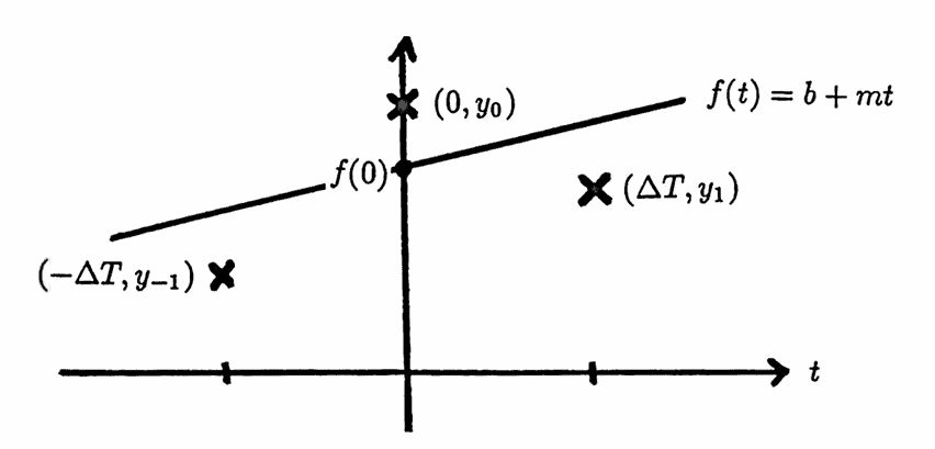
Nonrecursive filter example: smoothing by 3s

By defining

$$ \begin{gather} f_1(t) := 1\ \ \text{and}\ \ f_2(t) := t\,,\cr\cr {\bf t} = \begin{bmatrix}-\Delta T\\ 0\\ \Delta T \end{bmatrix} \ \ \ \text{and}\ \ \ {\bf y} = \begin{bmatrix} y_{-1}\\ y_0\\ y_1 \end{bmatrix}\,,\cr\cr {\bf f}_1({\bf t}) := \begin{bmatrix} f_1(-\Delta T)\\ f_1(0)\\ f_1(\Delta T) \end{bmatrix} = \begin{bmatrix} 1\\ 1\\ 1 \end{bmatrix}\cr\cr \text{and}\cr\cr {\bf f}_2({\bf t}) := \begin{bmatrix} f_2(-\Delta T)\\ f_2(0)\\ f_2(\Delta T) \end{bmatrix} = \begin{bmatrix} -\Delta T\\ 0\\ \Delta T \end{bmatrix}\,,\cr\cr {\bf X} = \bigl[ {\bf f}_1({\bf t})\ \ \vdots\ \ {\bf f}_2({\bf t}) \bigr] = \begin{bmatrix} 1 & -\Delta T\\ 1 & 0\\ 1 & \Delta T \end{bmatrix}\cr\cr \text{and}\cr\cr {\bf b} = \begin{bmatrix} b\\ m\end{bmatrix}\,, \end{gather} $$

and using the results from Section $2.2$, one obtains:

$$ \begin{align} {\bf b} &= ({\bf X}^t{\bf X})^{-1}{\bf X}^t{\bf y}\cr\cr &= \begin{bmatrix} 3 & 0\\ 0 & 2(\Delta T)^2\end{bmatrix}^{-1}{\bf X}^t{\bf y}\cr\cr &= \begin{bmatrix} \frac 13 & 0 \\ 0 & \frac 1{2(\Delta T)^2} \end{bmatrix} \begin{bmatrix} 1 & 1 & 1\\ -\Delta T & 0 & \Delta T \end{bmatrix} \begin{bmatrix} y_{-1}\\ y_0\\ y_1\end{bmatrix}\cr\cr &= \begin{bmatrix} \frac13(y_{-1} + y_0 + y_1)\\ \frac 1{2\Delta T}(y_1 - y_{-1}) \end{bmatrix} \end{align} $$

Then, $\,f_0 = b = \frac 13(y_{-1} + y_0 + y_1)\,.$ Thus, the current filter value is found by averaging the immediate past, current, and immediate future data values. Generalizing this process gives the filter

$$ f_n = \frac 13(y_{n-1} + y_n + y_{n+1})\ , $$

which is nonrecursive, with $\,c_{-1} = c_0 = c_1 = \frac 13\,.$ Not surprisingly, this filter is called a moving average filter, or smoothing by $3$’s.

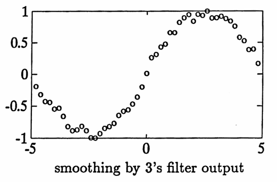
Example: Applying the Smoothing by $3$’s Filter

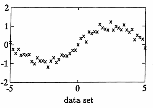
A data set, generated by $\,y(t) = t^2\,$ and then corrupted with noise, is plotted below using the plot symbol ‘x’. The smoothing by $3$’s filter is applied, and the filtered output is plotted with ‘o’.

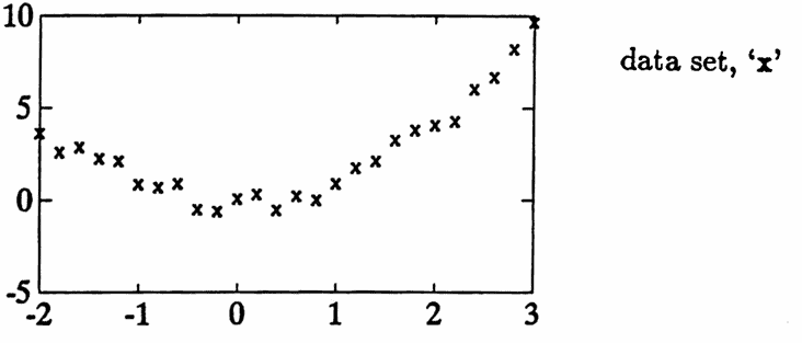
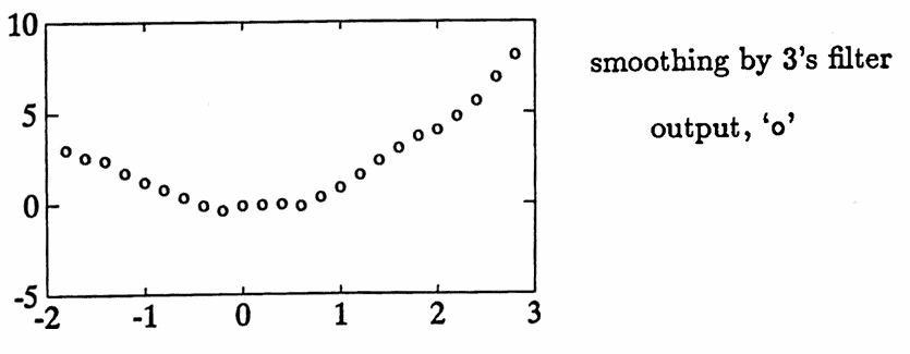
Note that the filtered curve is certainly ‘smoother’, so the filter is appropriately named. A better understanding of what this filter does will come from studying its corresponding transfer function in Section $3.2\,.$

The filter lag problem

Consider applying the smoothing by $3$’s filter to the data values from a finite data set $\,\{(t_i,y_i)\}_{i=1}^N\,.$ Since computation of filter value $\,f_n\,$ requires knowledge of the values $\,y_{n-1}\,,$ $\,y_n\,$ and $\,y_{n+1}\,,$ it is not possible to compute $\,f_1\,$ (since $\,y_0\,$ is unknown) or $\,f_N\,$ (since $\,y_{N+1}\,$ is unknown).

This inability to get filter output corresponding to the entire data set becomes worse as the number of nonzero coefficients in the filter increases.

Window of coefficients

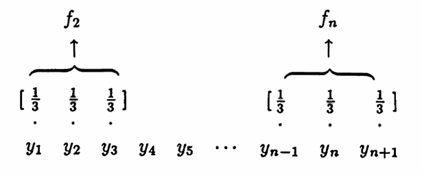
In filter literature, the smoothing by $3$’s filter is often described via the phrase: ‘we are looking at the data through the window $\,[\frac 13\ \frac 13\ \frac 13]\,$’. One imagines this ‘window’ moving successively to the right through the data values, producing the filtered values, as illustrated below.

A note regarding the filter coefficients

Suppose that the sum of the filter coefficients for a nonrecursive filter is $\,1\,,$ that is:

$$ \sum_k c_k = 1 $$

(This is true in the previous example, since $\,\frac 13 + \frac13 + \frac13 = 1\,.$) Then, when a constant function $\,y_n := K\,$ is input to the filter, the same constant emerges as the filter output:

$$ \begin{align} f_n &= \sum_k c_k\,y_{n-k}\cr\cr &= \sum_k c_k(K)\cr\cr &= K\sum_k c_k\cr\cr &= K(1) = K \end{align} $$

A MATLAB function for applying nonrecursive filters

A MATLAB function for applying nonrecursive filters is given next. It is assumed that the nonrecursive filter is of the form

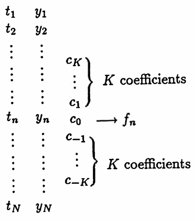
$$ f_n = \sum_{k = -K}^K c_k\,y_{n-k} $$

for a positive integer $\,K\,$; some of the coefficients $\,c_k\,$ may equal zero. There are $\,2K+1\,$ filter coefficients: $\,c_K,\ldots,c_1,c_0,c_{-1},\ldots,c_{-K}\,.$

MATLAB IMPLEMENTATION: Applying a Nonrecursive Filter

MATLAB function: nonrec(D,FC)

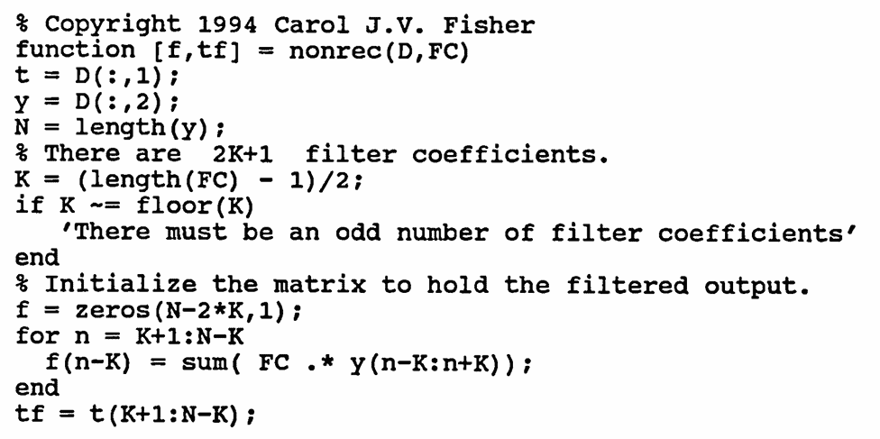
The MATLAB function nonrec applies the nonrecursive filter

$$ f_n = \sum_{k=-K}^K c_k\,y_{n-k} $$

to the data values in a data set D . The filter coefficients are stored in a column vector FC .

To use the function, type:
[f tf] = nonrec(D,FC);

Required Inputs

A data set $\,\{(t_i,y_i)\}_{i=1}^N\,$ is required, with a uniform time list. Here, $\,N\,$ is a positive integer that gives the number of data points.
The time values are stored in an $N$-column vector called t , and the corresponding data values are stored in an $N$-column vector called y . Then, D = [t y] is the $\,N \times 2\,$ matrix containing the data set.
The $\,2K+1\,$ real number filter coefficients $\,c_K,\ldots,c_1,c_0,c_{-1},\ldots,c_{-K}\,$ must be stored, in the indicated order, in a column vector called FC (for ‘Filter Coefficients’). Here, $\,K\,$ is a nonnegative integer.
It must be the case that $\,N \gt 2K\,$ if any filter output is to be observed. Otherwise, the output matrices f and tf will be empty.

filter coefficients acting on a data set

Output

The function outputs $\,2\,$ column vectors, f and tf .

The vector f contains the filtered output. Filtered output $\,f_n\,$ corresponds to data value $\,y_n\,.$

The vector tf contains the time values for the filtered output ( tf stands for ‘time for filtered output’). Filtered output $\,f_n\,$ corresponds to time value $\,t_n\,.$

The first and last $\,K\,$ values in y cannot be processed, due to filter lag. Therefore, the length of f (and tf ) is $\,N - 2K\,.$

Plotting the original data versus the filtered data

The original data can be plotted versus the filtered data with the commands:
plot(t,y,'x)
hold
plot(tf,f,'o')

Source code

The source code for the function nonrec is given next.

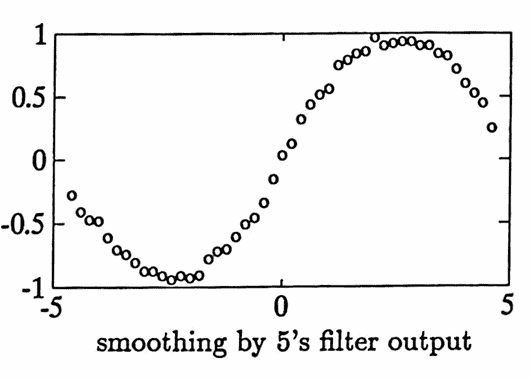
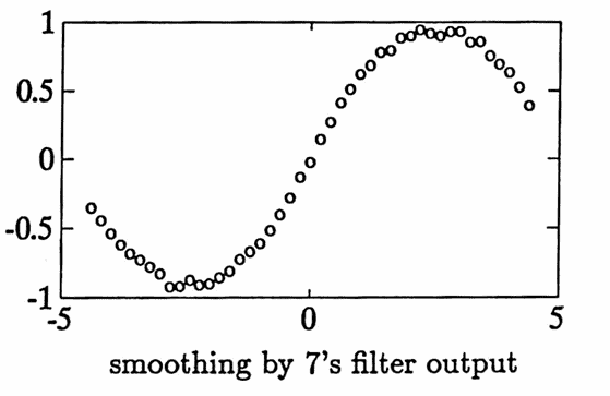
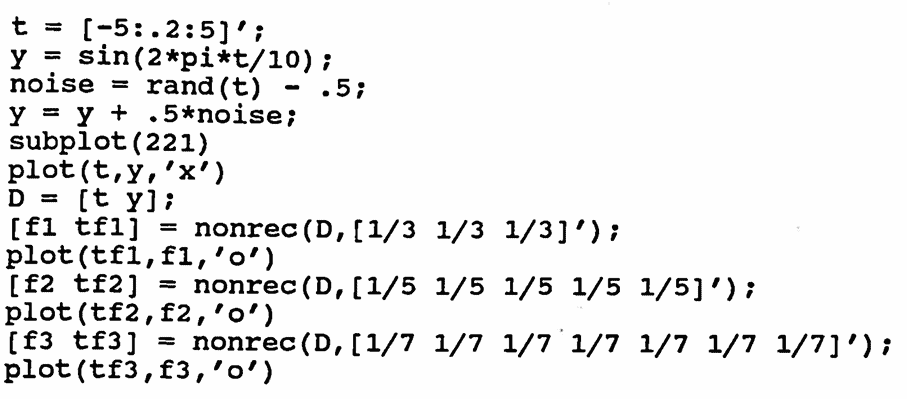
Octave requires endfunction as the last line.

EXAMPLE

The next example illustrates the use of nonrec . A noisy data set is constructed. Three filters are then applied:

the smoothing by $3$’s filter (with window $\,\frac13[1\ 1\ 1]\,$);
the smoothing by $5$’s filter (with window $\,\frac 15[1\ 1\ 1\ 1\ 1]\,$); and
the smoothing by $7$’s filter (with window $\,\frac 17[1\ 1\ 1\ 1\ 1\ 1\ 1]\,$).

Observe that the filtered data does appear to become increasingly ‘smoother’. Also notice the increasing filter lag problem.

A further understanding of these filters comes from studying their corresponding transfer functions, which is the subject of the next section.

Example: applying three different smoothing filters

Octave requires:
noise = rand(size(t)) - .5;