3.3 Designing and Improving Filters
The previous section investigated the problem: given a symmetric nonrecursive filter, find its transfer function. The current section shows how to go from a desired transfer function to a symmetric nonrecursive filter. The Fourier series of the desired transfer function plays an important role in this process.
Continuous Fourier series results were reviewed in Section $1.6$. For the current purpose, it is easiest to employ the equivalent complex form of the Fourier series. The relevant results are summarized below. The interested reader is referred to [Ham, $95$–$99$] for additional information.
Let $\,g\,$ be a periodic real-valued function of one real variable. Suppose that $\,g\,$ is piecewise continuous on $\,\Bbb R\,,$ and has fundamental period $\,P\,.$
The complex Fourier series of $\,g\,$, denoted by $\,\text{Four}(g)\,,$ is the infinite sum
$$ \text{Four}(g)(t) := \sum_{k=-\infty}^\infty C_k\,e^{i\frac{2\pi kt}P}\ , $$where:
$$ C_k = \frac 1P\int_P e^{-i\frac{2\pi kt}P}\,g(t)\,dt $$The coefficients $\,C_k\,$ are related to the coefficients $\,a_k\,$ and $\,b_k\,$ by:
$$ \begin{align} C_k &= \frac{a_{(-k)} + ib_{(-k)}}2\ \ \text{for}\ \ k\lt 0\ ,\cr\cr C_0 &= \frac{a_0}2\ ,\cr\cr C_k &= \frac{a_k - ib_k}2\ \ \text{for}\ \ k\gt 0 \end{align} $$If $\,g\,$ is an even function ($\,g(-t) = g(t)\,$ for all $\,t\,$), then $\,b_k = 0\,$ for $\,1\le k\lt \infty\,,$ and hence:
$$ C_k = \cases{ \frac{a_{(-k)}}2 & \text{for}\ \ k\lt 0\cr\cr \frac{a_k}2 & \text{for}\ \ k\ge 0 } $$In particular, if $\,g\,$ is even, then all values of $\,C_k\,$ are real numbers, and $\,C_k = C_{(-k)}\,$ for all integers $\,k\,.$
In order to compare a transfer function $\,\tilde H\,$ (as a function of cyclic frequency) with its complex Fourier series representation, it is rewritten as follows:
$$ \begin{align} &\tilde H(f)\cr\cr &\quad := \sum_{k=-K}^K c_k\,e^{-i2\pi kf\Delta T}\cr\cr &\quad = \sum_{\ell = K}^{-K} c_{(-\ell)}\,e^{i2\pi \ell f \Delta T}\ \ (\ell := -k)\cr\cr &\quad = \sum_{k=-K}^K c_{(-k)}\,e^{i2\pi kf\Delta T} \tag{1} \end{align} $$Recall from the previous section that $\,\tilde H\,$ has period $\,\frac 1{\Delta T}\,.$ Therefore, the complex Fourier series for $\,\tilde H\,$ is given by:
$$ \begin{align} &\text{Four}(\tilde H)(f)\cr\cr &\quad = \sum_{k=-\infty}^{\infty} C_k\,e^{i\frac{2\pi kf}{1/\Delta T}}\cr\cr &\quad = \sum_{k=-\infty}^\infty C_k\,e^{i2\pi kf\Delta T}\ \ \tag{2} \end{align} $$By comparing ($1$) and ($2$), it is apparent that the truncated Fourier series will approximate the transfer function, provided that $\,C_k = c_{(-k)}\,$ for $\,k = -K,\ldots,K\,.$
The procedure for finding filter coefficients from a given (desired) transfer function is summarized next:
- Let $\,\Delta T\,$ be a given positive number, representing the uniform spacing in the time list of a data set to be processed. Let $\,\tilde H\,$ denote a desired transfer function on the interval of frequencies $\,[0,\frac 1{2\Delta T}]\,.$
-
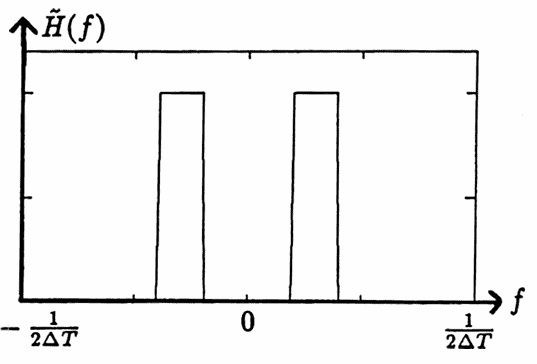
Extend $\,\tilde H\,$ to $\,[-\frac 1{2\Delta T},\frac 1{2\Delta T}]\,$ via:
$$ \tilde H(-t) = \tilde H(t)\ \ \text{for}\ \ t\in [0,\frac 1{2\Delta T}] $$(See the diagram below.) Call this extension by the same name.
-
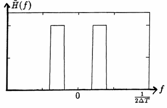
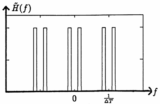
Extend $\,\tilde H\,$ periodically to all of $\,\Bbb R\,.$ (See the diagram below.) That is, define
$$ \tilde H\left( t + k\bigl( \frac 1{\Delta T} \bigr) \right) := \tilde H(t) $$for all integers $\,k\,,$ and for all $\,t \in [-\frac 1{2\Delta T},\frac 1{2\Delta T}]\,.$ Call this extension by the same name. The resulting function $\,\tilde H\,$ is even, with fundamental period $\,\frac 1{\Delta T}\,.$
-
Since $\,\tilde H\,$ is even, its complex Fourier series coefficients $\,C_k\,$ are real numbers, and $\,C_k = C_{(-k)}\,$ for all integers $\,k\,.$ For $\,k\ge 0\,,$
$$ C_k = \frac{a_k}2\ , $$where
$$ \begin{align} a_k &=\frac 2P\int_P \tilde H(f)\cos\frac{2\pi kf}P\,df\ \ \text{(see $\S$1.6)}\cr\cr &= 2\Delta T\int_{-\frac 1{2\Delta T}}^{\frac 1{2\Delta T}} \tilde H(f)\cos(2\pi kf\Delta T)\,df\cr &\qquad\qquad\qquad \text{(since $\,P = \frac 1{\Delta T}\,$)}\cr\cr &= 4\Delta T\int_0^{\frac 1{2\Delta T}} \tilde H(f)\cos(2\pi kf\Delta T)\,df\cr &\qquad\qquad\qquad \text{(since $\,\tilde H\,$ is even)}\tag{3} \end{align} $$
-
For a positive integer $\,K\,,$ the coefficients $\,c_k\,$ given by
$$ c_k = c_{-k} = C_k\ \ \text{for}\ \ k = 0,\ldots,K $$will give a symmetric nonrecursive filter
$$ f_n = \sum_{k=-K}^K c_k\,y_{n-k} $$with a transfer function that approximates $\,\tilde H(f)\,.$ In general, the greater the value of $\,K\,,$ the better the approximation.
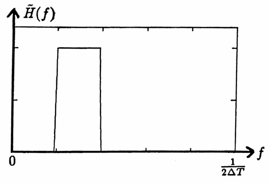
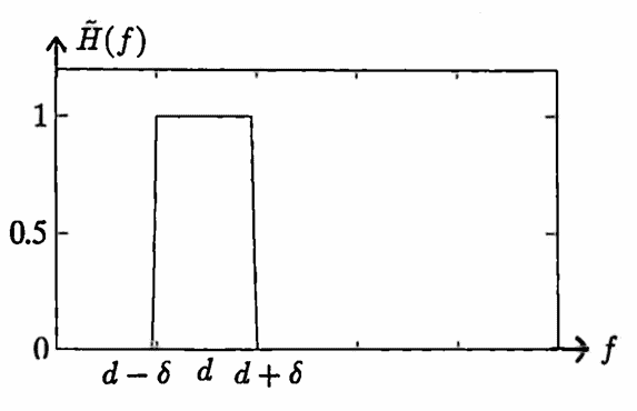
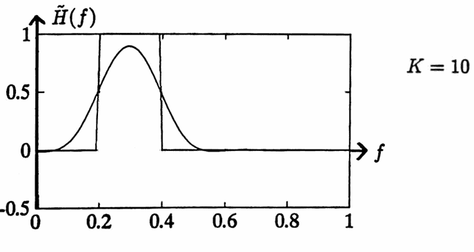
The procedure just described is illustrated next. Let $\,\Delta T = 0.5\,,$ so that $\,\frac 1{2\Delta T} = 1\,.$ A transfer function is desired that will pass the frequencies in an interval $\,[d-\delta\,,\,d+\delta] \subset [0,\frac 1{2\Delta T}]\,,$ and suppress all other frequencies. Such a filter is called a band-pass filter. The desired transfer function is shown below on $\,[0,\frac 1{2\Delta T}]\,.$
Using ($3$):
$$ \begin{align} a_k &= 4\Delta T\int_0^{\frac 1{2\Delta T}} \tilde H(f)\,\cos(2\pi kf\Delta T)\,df\cr\cr &= 4(0.5)\int_0^1 \tilde H(f)\,\cos(2\pi kf(0.5))\,df\cr\cr &= 2 \int_{d-\delta}^{d+\delta} (1)\cos(k\pi f)\,df\cr\cr &= \frac 2{k\pi}[\sin(k\pi(d+\delta)) - \sin(k\pi(d-\delta))]\ ,\ \ \text{for}\ \ k\gt 0 \end{align} $$Also:
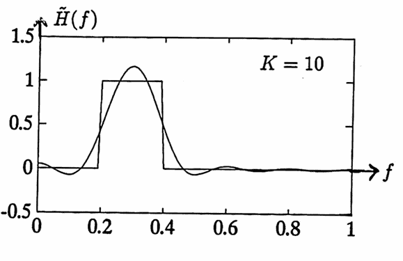
$$ \begin{align} a_0 &= 4\Delta T\int_{d-\delta}^{d+\delta} (1)\,df\cr\cr &= 4(0.5)(2\delta) = 4\delta \end{align} $$Let $\,d = 0.3\,,$ $\,\delta = 0.1\,,$ and $\,K = 10\,.$ The resulting symmetric nonrecursive filter has coefficients:
$$ \begin{align} &(c_0,c_1,\ldots,c_{10})\cr\cr &\quad = \bigl( \frac{a_0}2,\frac{a_1}2,\ldots,\frac{a_{10}}2 \bigr)\cr\cr &\quad \approx (0.2,\,0.1156,\,-0.0578,\,-0.1633,\cr &\qquad -0.1225,\,0\,,0.0816,\,0.0700,\cr &\qquad 0.0145,\,-0.0128,\,0) \end{align} $$The transfer function for this filter is shown below, superimposed with the ‘ideal’ transfer function.
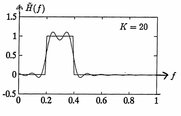
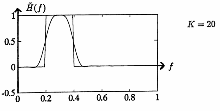
Now, increase $\,K\,$ to $\,20\,,$ keeping all other parameters the same. The transfer function of the resulting symmetric nonrecursive filter is shown below, superimposed with the ‘ideal’ transfer function.
The ‘ripples’ that appear in the transfer functions can be ‘smoothed’ by a process called Lanczos smoothing.
Lanczos is credited with observing that the ‘ripple’ in a truncated Fourier series has approximately the period of the last term kept in the series. He argued that smoothing the partial sum by integrating (averaging) over this period would remove the main effects of the ripple. This procedure is discussed next. The interested reader is referred to [Ham, $109$–$112$] for additional information.
Consider the truncation
$$ T(f) := \sum_{k=-K}^K C_k\,e^{i2\pi kf\Delta T} $$of the infinite sum
$$ \text{Four}(\tilde H)(f) := \sum_{k=-\infty}^\infty C_k\,e^{i2\pi kf\Delta T} $$The last terms kept correspond to indices $\,k = K\,$ and $\,k = -K\,,$ with corresponding period $\,\frac 1{K\Delta T}\,.$ Define a ‘smoothed’ function $\,S(f)\,,$ obtained by replacing the number $\,T(f)\,$ with the average value of the function $\,T\,$ over an interval of length $\,\frac 1{K\Delta T}\,$ centered at $\,f\,$:
$$ \begin{align} S(f) &:=\frac 1{1/(K\Delta T)}\int_{f-\frac 1{2K\Delta T}}^{f+\frac 1{2K\Delta T}} T(f)\,df\cr\cr &= \frac 1{1/(K\Delta T)}\int_{f-\frac 1{2K\Delta T}}^{f+\frac 1{2K\Delta T}} \sum_{k=-K}^K C_k\,e^{i2\pi kf\Delta T}\,df\cr\cr &= K\Delta T\sum_{k=-K}^K C_k \int_{f-\frac 1{2K\Delta T}}^{f+\frac 1{2K\Delta T}} e^{i2\pi kf\Delta T}\,df\cr\cr &= K\Delta T\sum_{k=-K}^K \frac{C_k}{\pi k\Delta T}\, e^{i2\pi kf\Delta T} \left[ \frac{ e^{i(\pi k/K)} - e^{-i(\pi k/K)}}{2i} \right]\cr\cr &= K\sum_{k=-K}^K \frac{C_k}{\pi k}\,e^{i2\pi kf\Delta T}\sin(\pi k/K)\cr\cr &= \sum_{k=-K}^K C_k \left[ \frac{\sin(\pi k/K)}{\pi k/K} \right]\, e^{i2\pi kf\Delta T} \end{align} $$Observe that in the resulting function $\,S(f)\,,$ the $\,k^{\text{th}}\,$ term of $\,T(f)\,$ has been scaled by the number:
$$ \frac{\sin(\pi k/K)}{\pi k/K} $$These scaling factors are commonly called the sigma factors. Observe that:
$$ \begin{align} \frac{\sin\bigl( \pi(-k)/K\bigr)}{\pi(-k)/K} &= \frac{-\sin(\pi k/K)}{-\pi k/K}\cr\cr &= \frac{\sin(\pi k/K)}{\pi k/K} \end{align} $$Also, when $\,k = 0\,,$ the sigma factor is defined to equal $\,1\,,$ since:
$$ \lim_{k\rightarrow 0} \frac{\sin(\pi k/K)}{\pi k/K} = 1 $$The distinct values of the sigma factors are shown below, when $\,K = 10\,$:
| $k$ | sigma factor |
|---|---|
| $0$ | $1$ |
| $1$ | $0.9836$ |
| $2$ | $0.9355$ |
| $3$ | $0.8584$ |
| $4$ | $0.7568$ |
| $5$ | $0.6366$ |
| $6$ | $0.5046$ |
| $7$ | $0.3679$ |
| $8$ | $0.2339$ |
| $9$ | $ 0.1093$ |
| $10$ | $0$ |
The transfer functions of the previous example, after Lanczos smoothing is applied, become:
MATLAB IMPLEMENTATION: Finding a Symmetric Nonrecursive Filter Corresponding to a Desired Transfer Function
The MATLAB function findfil , with source code given below, computes the coefficients of a symmetric nonrecursive filter corresponding to a desired transfer function.
To use the function, type:
[C,Hf,f] = findfil(tH,H,K,dT,smooth);
The required inputs are:
- A positive number $\,\Delta T\,$ that represents the uniform spacing in the time list of a data set to be processed. The MATLAB variable dT contains the desired value of $\,\Delta T\,.$
- A description of the desired transfer function on the interval $\,[0,\frac 1{2\Delta T}]\,.$ The description must be contained in two column vectors, tH and H , of equal length: the column vector tH contains equally-spaced entries from the interval $\,[0,\frac 1{2\Delta T}]\,,$ and H contains the corresponding desired values of the transfer function.
- K is a positive integer that gives the last term to be kept in the truncated Fourier series. The resulting nonrecursive filter will have K$+ 1\,$ distinct filter coefficients, $\,c_0,c_1,\ldots,c_K\,.$
- If Lanczos smoothing is desired, set smooth = 1 . Any other value for smooth , or removing this variable from the input list, gives an unsmoothed filter.
The function outputs three column vectors, C , Hf , and f .
- The column vector C contains the K$+ 1\,$ distinct coefficients $\,c_0,c_1,\ldots,c_K\,$ of the corresponding nonrecursive filter.
-
The column vectors f and Hf contain the information necessary to plot the transfer function corresponding to the nonrecursive filter (which is an approximation to the desired transfer function). This approximation can be plotted, superimposed with the actual transfer function, via the commands:
plot(f,Hf)
hold
plot(tH,H)
The source code for the function findfil is given next:
function [C,Hf,f] = findfil(tH,H,K,dT,smooth)
 if nargin==4
   smooth = 0;
 end
 N = length(tH);
 P = tH(N);
 C = zeros(K+1,1);
 C(1) = (1/N)*sum(H);
 for k = 2:(K+1)
   tvec = (2*pi*(k-1)*dT)*tH;
   cosv = cos(tvec);
   C(k) = (1/N)*sum(H .* cosv);
 end
 if smooth==1
   k = [1:K]';
     k = pi*k/K;
     sigma = sin(k) ./ k;
     C(2:K+1) = sigma .* C(2:K+1);
 end
 [Hf,f] = transfct(C,dT);
The MATLAB function symtofc (‘symmetric to filter coefficients’) converts the $\,K+1\,$ distinct coefficients $\,c_0,c_1,\ldots,c_K\,$ from a nonrecursive symmetric filter, to the full set of coefficients
$$ c_{-K},\ldots,c_{-1},c_0,c_1,\ldots,c_K $$(where $\,c_{-k} = c_k\,$), for use in the function nonrec .
To use the function, type:
FC = symtofc(C);
 function FC = symtofc(C);
 K = length(C) - 1;
 FC = flipud(C(2:(K+1)));
 FC = [FC;C];
The input is a column vector C containing the coefficients $\,c_0,c_1,\ldots,c_K\,.$
The output is a column vector FC containing the full set of coefficients $\,c_{-K},\ldots,c_{-1},c_0,c_1,\ldots,c_K\,.$
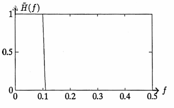
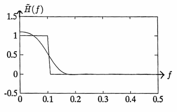
The following diary of an actual MATLAB session illustrates the use of the functions findfil and symtofc . Here, a low-pass filter (which passes low frequencies, and suppresses high frequencies) is designed, corresponding to spacing $\,\Delta T = 1\,.$ The designed filter is then used to process a ‘known unknown’.
% Construct the desired transfer function:
 tH1 = [0:.01:.10]';
 tH2 = [.11:.01:.5]';
 y1 = ones(tH1);
 y2 = zeros(tH2);
 tH = [tH1;tH2];
 H = [y1;y2] ;
% Graph the desired transfer function:
 plot(tH,H)
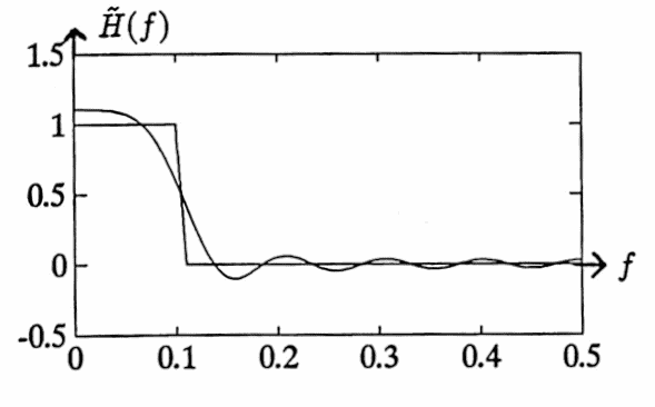
% Find a corresponding unsmoothed filter,
%   dT = 1, K = 10:
 [C,Hf,f] = findfil(tH,H,10,1);
% Plot the transfer function
%   of the corresponding filter,
%   superimposed with the ideal transfer filter:
 plot(f,Hf)
 hold
Current plot held

 plot(tH,H)
 hold

Current plot released
% Now, find a corresponding smoothed filter,
%   dT = 1, K = 10:
 [C,Hf,f] = findfil(tH,H,10,1,1);
 plot(f,Hf)
 hold

Current plot held

 plot(tH,H)
 hold

Current plot released
C
% Here are the smoothed filter coefficients
% c0,c1,...,c10 :
C =
0.2157
0.1978
0.1506
0.0905
0.0359
0.0000
-0.0143
-0.0129
-0.0055
-0.0002
0.0000
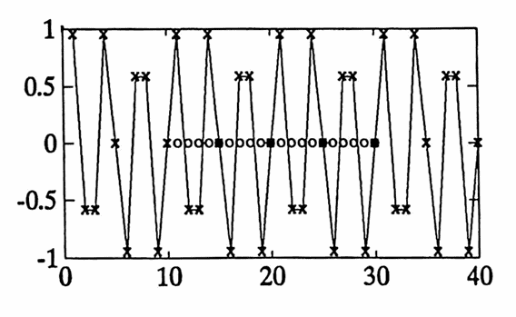
t = [1:40]';
y = sin(2*pi*.3*t)
plot(t,y)
hold
Current plot held
plot(t,y,'x')
FC = symtofc(C);
D = [t y];
[f,tf] = nonrec(D,FC);
plot(tf,f,'o')