2.6 Discrete Fourier Series and the Periodogram
Suppose $\,\{(t_i,y_i)\}_{i=1}^N\,$ is a data set with a uniform time list; let $\,\Delta T\gt 0\,$ be such that $\,t_{k+1} - t_k = \Delta T\,$ for $\,k = 1,\ldots,N-1\,.$
If it is suspected that this data set has at least one periodic component, but there is no specific conjecture as to its period or form, then the discrete Fourier series corresponding to the data may give useful information regarding the periodic component.
The reader should compare the results in this section with the corresponding results regarding continuous Fourier series, which were reviewed in Section 1.6.
The next few results will lead to the definition of the discrete Fourier series.
Consider the constant function $\,f(t) \equiv 1\,,$ and the functions
$$ \sin\frac{2\pi kt}P\ \ \text{and}\ \ \cos\frac{2\pi kt}P $$for $\,k = 1,\ldots,K\,,$ where $\,P\,$ is a positive real number, and $\,K\,$ is a positive integer. This collection of $\,2K +1\,$ functions is mutually orthogonal with respect to the time values $\,t_1,\ldots,t_N\,,$ where $\,N \gt 1\,$ is a positive integer, if the following conditions are met:
- The list $\,(t_1,t_2,\ldots,t_N)\,$ is uniform with $\,\Delta T = \frac PN\,,$ and
- $N\ge 2K + 1\,.$
Proof of Theorem $1$
Recalling the definition of mutually orthogonal functions from Section $2.3\,,$ it must be shown that:
$$ \begin{gather} \sum_{n=1}^N \cos\frac{2\pi jt_n}P\,\cos\frac{2\pi kt_n}P = 0\,,\ \ j,k = 1,\ldots,K\,,\ j\ne k\,,\tag{1}\cr\cr \sum_{n=1}^N \sin\frac{2\pi jt_n}P\,\sin\frac{2\pi kt_n}P = 0\,,\ \ j,k = 1,\ldots,K\,,\ j\ne k\,,\tag{2}\cr\cr \sum_{n=1}^N \sin\frac{2\pi jt_n}P\,\cos\frac{2\pi kt_n}P = 0\,,\ \ j,k = 1,\ldots,K\,, \ \ \text{and}\tag{3}\cr\cr \sum_{n=1}^N \cos\frac{2\pi kt_n}P = \sum_{n=1}^N \sin\frac{2\pi kt_n}P = 0\,,\ \ k = 1,\ldots,K\,. \tag{4} \end{gather} $$The proof makes use of the identities
$$ \begin{gather} \cos t = \frac 12(e^{it} + e^{-it})\cr\cr \text{and}\cr\cr \sin t = \frac 1{2i}(e^{it} - e^{-it})\ ,\cr\cr \forall\ \ t\in\Bbb R\,, \end{gather} $$and Proposition $2$ from Section $1.6\,,$ which states that
$$ \begin{gather} \sum_{n=0}^{N-1} e^{2\pi ki(\frac nN)} = 0\cr \text{and}\cr \sum_{n=0}^{N-1} e^{-2\pi ki(\frac nN)} = 0 \end{gather} $$whenever $\,N\,$ and $\,k\,$ are positive integers with $\,N \gt 1\,,$ and $\,1\le k\le N-1\,.$ Since the time list is uniform with spacing $\,\frac PN\,,$ one can write $\,t_n = t_1 + (n-1)\frac PN\,$ for $\,n = 1,\ldots,N\,.$ Let $\,j,k = 1,\ldots,K\,$ with $\,j\ne k\,.$ Then:
$$ \begin{align} &\sum_{n=1}^N \cos\frac{2\pi jt_n}P\,\cos\frac{2\pi kt_n}P\cr\cr &\quad = \sum_{n=1}^N\cos\left( \frac{2\pi jt_1}P + \frac{2\pi j(n-1)}N \right) \cos\left( \frac{2\pi kt_1}P + \frac{2\pi k(n-1)}N \right)\cr\cr &\quad = \sum_{n=0}^{N-1} \cos\left( \frac{2\pi jt_1}P + \frac{2\pi jn}N \right) \cos\left( \frac{2\pi kt_1}P + \frac{2\pi kn}N \right)\cr\cr &\quad = \frac 14 \sum_{n=0}^{N-1} \left( e^{i(\frac{2\pi jt_1}P + \frac{2\pi jn}N)} + e^{-i(\frac{2\pi jt_1}P + \frac{2\pi jn}N)} \right) \left( e^{i(\frac{2\pi kt_1}P + \frac{2\pi kn}N)} + e^{-i(\frac{2\pi kt_1}P + \frac{2\pi kn}N)} \right) \end{align} $$To simplify notation, let $\,C_j := \frac{2\pi jt_1}P\,$ and $\,C_k := \frac{2\pi kt_1}P\,.$ Observe that both $\,C_j\,$ and $\,C_k\,$ are independent of the index of summation, $\,n\,.$ With this notation:
$$ \begin{align} &\frac 14 \sum_{n=0}^{N-1} \left( e^{i(\frac{2\pi jt_1}P + \frac{2\pi jn}N)} + e^{-i(\frac{2\pi jt_1}P + \frac{2\pi jn}N)} \right) \left( e^{i(\frac{2\pi kt_1}P + \frac{2\pi kn}N)} + e^{-i(\frac{2\pi kt_1}P + \frac{2\pi kn}N)} \right)\cr\cr &\quad = \frac 14 \sum_{n=0}^{N-1} \left( e^{i(C_j + \frac{2\pi jn}N)} + e^{-i(C_j + \frac{2\pi jn}N)} \right) \left( e^{i(C_k + \frac{2\pi kn}N)} + e^{-i(C_k + \frac{2\pi kn}N)} \right)\cr\cr &\quad = \frac 14 \sum_{n=0}^{N-1} \left( e^{iC_j}e^{i\frac{2\pi jn}N} + e^{-iC_j}e^{-i\frac{2\pi jn}N} \right) \left( e^{iC_k}e^{i\frac{2\pi kn}N} + e^{-iC_k}e^{-i\frac{2\pi kn}N} \right)\cr\cr &\quad = \overbrace{\frac 14e^{i(C_j+C_k)}\sum_{n=0}^{N-1} e^{2\pi(j+k)i(\frac nN)}}^{\text{first sum}} + \overbrace{\frac 14e^{-i(C_j+C_k)}\sum_{n=0}^{N-1} e^{-2\pi(j+k)i(\frac nN)}}^{\text{second sum}}\cr\cr &\qquad + \overbrace{\frac 14e^{i(C_j-C_k)}\sum_{n=0}^{N-1} e^{2\pi(j-k)i(\frac nN)}}^{\text{third sum}} + \overbrace{\frac 14e^{-i(C_j-C_k)}\sum_{n=0}^{N-1} e^{-2\pi(j-k)i(\frac nN)}}^{\text{fourth sum}} \tag{5} \end{align} $$Since $\,j\,$ and $\,k\,$ take on positive integer values between $\,1\,$ and $\,K\,$ with $\,j\ne k\,,$ and since $\,N \ge 2K + 1\,,$ it follows that:
$$ \begin{align} 3 &\le j + k\cr &\le K + (K-1)\cr &= 2K-1\cr &\le (N-1) - 1 \cr &= N - 2 \end{align} $$In particular, $\,1 \le j + k \le N — 1\,,$ so by Proposition $2$, the first and second sums in equation ($5$) vanish.
Without loss of generality, suppose that $\,j \gt k\,.$ Then:
$$ \begin{align} 1 &\le j - k\cr\cr &\le K - 1\cr\cr &\le \frac{N-1}2 - 1\cr\cr &\lt N - 1 \end{align} $$In particular, $\,1 \le j-k \le N-1\,,$ so the third and fourth sums also vanish. This completes the proof of ($1$). The same technique applies, with obvious changes, to prove ($2$).
To verify ($3$), drop the restriction that $\,j\,$ and $\,k\,$ be nonequal, and compute:
$$ \begin{align} &\sum_{n=1}^N \sin\frac{2\pi jt_n}P\,\cos\frac{2\pi kt_n}P\cr\cr &\quad = \sum_{n=0}^{N-1} \frac1{2i}\left( e^{i(C_j+\frac{2\pi jn}N)} - e^{-i(C_j+\frac{2\pi jn}N)} \right) \frac1{2}\left( e^{i(C_k+\frac{2\pi kn}N)} + e^{-i(C_k+\frac{2\pi kn}N)} \right)\cr\cr &\quad = \overbrace{\frac 1{4i}e^{i(C_j+C_k)}\sum_{n=0}^{N-1} e^{2\pi(j+k)i(\frac nN)}}^{\text{first sum}} - \overbrace{\frac 1{4i}e^{-i(C_j+C_k)}\sum_{n=0}^{N-1} e^{-2\pi(j+k)i(\frac nN)}}^{\text{second sum}}\cr\cr &\qquad + \overbrace{\frac 1{4i}e^{i(C_j-C_k)}\sum_{n=0}^{N-1} e^{2\pi(j-k)i(\frac nN)}}^{\text{third sum}} - \overbrace{\frac 1{4i}e^{-i(C_j-C_k)}\sum_{n=0}^{N-1} e^{-2\pi(j-k)i(\frac nN)}}^{\text{fourth sum}} \tag{6} \end{align} $$If $\,j\ne k\,,$ then previous arguments show that all four sums vanish. If $\,j = k\,,$ then the last two sums cancel, since $\,C_j = C_k\,$ and $\,j - k = 0\,.$ Also, if $\,j = k\,,$ then $\,j + k = 2j \le 2K \le N - 1\,,$ so the first two sums vanish.
Similar arguments show that equations ($4$) are true. $\blacksquare$
The restriction $\,N \ge 2K +1\,$ in Theorem $1$ is as good as possible; that is, no smaller value of $\,N\,$ works. In particular, if $\,N = 2K\,$ and $\,j = k = K\,,$ then the condition
$$ \sum_{n=1}^N \sin\frac{2\pi jt_n}P\,\cos\frac{2\pi kt_n}P = 0\,, \ \ j,k = 1,\ldots,K $$holds if and only if $\,\displaystyle \frac{4Kt_1}P\,$ is an integer.
Proof
It is first shown that when $\,N = 2K\,,$ Theorem $1$ is not true. Let $\,K = 2\,,$ $\,N = 4\,,$ $\,P = 2\pi\,,$ and $\,(t_1,t_2,t_3,t_4) = (\frac\pi 8, \frac{5\pi}8, \frac{9\pi}8, \frac{13\pi}8)\,.$ Let $\,j = k = 2\,.$ Then:
$$ \begin{align} &\sum_{n=1}^N \sin\frac{2\pi jt_n}P\,\cos\frac{2\pi kt_n}P\cr\cr &\quad = \sum_{n=1}^4 \sin 2t_n\, \cos 2t_n\cr\cr &\quad = \sin\frac{\pi}4\,\cos\frac{\pi}4 + \sin\frac{5\pi}4\,\cos\frac{5\pi}4\cr &\qquad + \sin\frac{9\pi}4\,\cos\frac{9\pi}4 + \sin\frac{13\pi}4\,\cos\frac{13\pi}4\cr\cr &\quad = 4(\frac 12) \ne 0 \end{align} $$Next, it is shown that Theorem $1$ holds with $\,N \ge 2K+1\,$ replaced by the less restrictive requirement $\,N \ge 2K\,,$ if and only if $\,\frac{4Kt_1}P\,$ is an integer. It is only necessary to consider the case $\,N = 2K\,.$ When $\,N = 2K\,$ and $\,j \ne k\,,$ then
$$ 3 \le j+k \le K + (K-1) = 2K - 1 = N-1 $$and, for $\,j > k\,$:
$$ 1\le j - k \le K - 1 = \frac N2 - 1 \lt N - 1 $$Thus, equations ($1$) and ($2$) from Theorem $1$ still hold. Also, equation ($3$) holds whenever $\,j \ne k\,.$
Suppose that $\,j = k\,,$ and consider equation ($6$) from the proof of Theorem $1\,.$ The third and fourth sums cancel. If $\,j \lt K\,,$ then $\,j + k \lt 2K\,,$ so that $\,j + k \le N - 1\,,$ and the first and second sums vanish. If $\,j = k = K\,,$ then the first and second sums become:
$$ \begin{align} &\frac 1{4i}e^{i(C_j+C_k)}\sum_{n=0}^{N-1} e^{2\pi(j+k)i(\frac nN)} - \frac 1{4i}e^{-i(C_j+C_k)}\sum_{n=0}^{N-1} e^{-2\pi(j+k)i(\frac nN)}\cr\cr &\quad = \frac 1{4i}e^{2iC_K}\sum_{n=0}^{N-1} e^{4\pi Ki(\frac n{2K})} - \frac 1{4i}e^{-2iC_K}\sum_{n=0}^{N-1} e^{-4\pi Ki(\frac n{2K})}\cr\cr &\quad = \frac 1{4i}e^{2iC_K}\sum_{n=0}^{N-1} e^{2\pi in} - \frac 1{4i}e^{-2iC_K}\sum_{n=0}^{N-1} e^{-2\pi in}\cr\cr &\quad = \frac N{4i} \bigl( e^{2iC_K} - e^{-2iC_K}\bigr)\cr\cr &\quad = \frac N{4i}(2i\sin 2C_K) \tag{7} \end{align} $$Thus, ($7$) equals zero if and only if $\,\sin 2C_K\,$ equals zero, if and only if $\,2C_K\,$ is an integer multiple of $\,\pi\,.$ That is, it must be that
$$ 2C_K := 2\left(\frac{2\pi Kt_1}P\right) = \pi j $$for some integer $\,j\,$; that is, $\,\frac{4K t_1}P\,$ must be an integer. Note that if $\,\frac{t_1}P\,$ is an integer, or if $\,t_1 = 0\,,$ then equation ($7$) equals zero. In the counterexample given above, $\,\frac{4Kt_1}P = \frac{4(2)(\pi/8)}{2\pi} = \frac 12\,$ is not an integer. $\blacksquare$
Let the conditions of Theorem $1$ hold. Then:
$$ \sum_{n=1}^N \cos^2\frac{2\pi kt_n}P = \frac N2\,,\ \ k = 1,\ldots,K\ , $$and
$$ \sum_{n=1}^N \sin^2\frac{2\pi kt_n}P = \frac N2\,,\ \ k = 1,\ldots,K $$Proof
Let $\,k = 1,\ldots,K\,.$ Using ($5$) from Theorem $1$ with $\,j = k\,,$ one obtains:
$$ \begin{align} &\sum_{n=1}^N \cos^2\frac{2\pi kt_n}P\cr\cr &\quad = \frac 14 e^{i2C_k} \sum_{n=0}^{N-1} e^{2\pi(2k)i(\frac nN)} + \frac 14 e^{-i2C_k} \sum_{n=0}^{N-1} e^{-2\pi(2k)i(\frac nN)}\cr\cr &\qquad + \frac 14 (1) \sum_{n=0}^{N-1} (1) + \frac 14 (1) \sum_{n=0}^{N-1} (1) \end{align} $$Since $\,2k \le 2K \le N - 1\,,$ Proposition $2$ (Section $1.6$) implies that the first and second sums vanish, and thus:
$$ \sum_{n=1}^N \cos^2\frac{2\pi kt_n}P = \frac N4 + \frac N4 = \frac N2 $$A similar procedure verifies the second result. $\blacksquare$
Let $\,P\,$ be a positive real number, and let $\,N\,$ and $\,K\,$ be positive integers with $\, N \ge 2K + 1\,.$ Let $\,\{(t_i,y_i)\}_{i=1}^N\,$ be a data set, where the time list $\,(t_1,\ldots,t_N)\,$ is uniform with $\,\Delta T = \frac PN\,.$ Define:
$$ f(t) := a_0 + \sum_{k=1}^K \bigl( a_k\cos\frac{2\pi kt}P + b_k\sin\frac{2\pi kt}P \bigr) $$Then, the least-squares solution to
$$ \underset{a_k,\,b_k\in\Bbb R}{\text{min}}\, \sum_{n=1}^N \bigl( y_i - f(t_i) \bigr)^2 $$is given by:
$$ \begin{align} a_0 &= \frac 1N\sum_{n=1}^N y_n\,,\cr\cr a_k &= \frac 2N\sum_{n=1}^N y_n\cos\frac{2\pi kt_n}P\,,\ \ k = 1,\ldots,K\ ,\ \ \text{and}\cr\cr b_k &= \frac 2N\sum_{n=1}^N y_n\sin\frac{2\pi kt_n}P\,,\ \ k = 1,\ldots,K \end{align} $$Proof of Theorem $2$
Recalling results from Sections $2.2$ and $2.3$, the least-squares solution $\,{\bf b} = (a_0,a_1,\ldots,a_K,b_1,\ldots,b_K)\,$ is given by $\,{\bf b} = ({\bf X}^t{\bf X})^{-1}{\bf X}^t{\bf y}\,,$ where $\,\bf y\,$ is the column vector of data values:
$$ \begin{align} f_1(t) &\equiv 1\,,\cr\cr f_{k+1}(t) &= \cos\frac{2\pi kt}P \,,\ \ k = 1,\ldots,K\ ,\cr\cr f_{k+(K+1)}(t) &= \sin\frac{2\pi kt}P \,,\ \ k = 1,\ldots,K\ ,\cr\cr {\bf X}_{ij} &= f_j(t_i)\,,\ \ 1\le i\le N\,,\ \ 1\le j \le 2K + 1\,,\cr\cr \text{and}\cr\cr ({\bf X}^t{\bf X})_{ij} &= \sum_{n=1}^N f_i(t_n)\,f_j(t_n)\,,\ \ 1\le i,j\le 2K + 1 \end{align} $$By Theorem 1, the functions $\,\{f_k\}_{k=1}^{2K+1}\,$ are mutually orthogonal with respect to the given time values, so the matrix $\,{\bf X}^t{\bf X}\,$ is diagonal, with:
$$ \begin{align} &({\bf X}^t{\bf X})_{11} = N\,,\cr\cr &({\bf X}^t{\bf X})_{k+1,k+1}\cr &\quad= \sum_{n=1}^N \cos^2\frac{2\pi kt_n}P = \frac N2\,,\ \ k = 1,\ldots,K\,,\cr\cr &\text{and}\cr\cr &({\bf X}^t{\bf X})_{k+K+1,k+K+1}\cr &\quad= \sum_{n=1}^N \sin^2\frac{2\pi kt_n}P = \frac N2\,,\ \ k = 1,\ldots,K \end{align} $$Recall that the inverse of a diagonal matrix is easily found by taking the reciprocals of each diagonal entry. Thus:
$$ \bigl( ({\bf X}^t{\bf X})^{-1}\bigr)_{kk} = \begin{cases} \frac 1N & k = 1\\ \frac 2N & k = 2,\ldots,2K+ 1 \end{cases} $$The matrix product $\,{\bf b}\,$ is now computed:
$$ \begin{align} &{\bf b} = ({\bf X}^t{\bf X})^{-1}{\bf X}^t{\bf y}\cr\cr &\quad = \begin{bmatrix} \frac 1N & 0 & 0 & \cdots & 0\cr 0 & \frac 2N & 0 & \cdots & 0\cr 0 & 0 & \frac 2N & \cdots & 0\cr \vdots & \vdots & \vdots & \ddots & 0\cr 0 & 0 & 0 & \cdots & \frac 2N \end{bmatrix}\cr\cr &\qquad\ \ {\huge \bf \cdot} \begin{bmatrix} f_1(t_1) & f_1(t_2) & f_1(t_3) & \cdots & f_1(t_N)\cr f_2(t_1) & f_2(t_2) & f_2(t_3) & \cdots & f_2(t_N)\cr f_3(t_1) & f_3(t_2) & f_3(t_3) & \cdots & f_3(t_N)\cr \vdots & \vdots & \vdots & \cdots & \vdots\cr f_{2K+1}(t_1) & f_{2K+1}(t_2) & f_{2K+1}(t_3) & \cdots & f_{2K+1}(t_N) \end{bmatrix} \, \begin{bmatrix} y_1\cr y_2\cr y_3\cr \vdots\cr y_N \end{bmatrix} \cr\cr &\quad = \begin{bmatrix} \frac 1Nf_1(t_1) & \frac 1Nf_1(t_2) & \frac 1Nf_1(t_3) & \cdots & \frac 1Nf_1(t_N)\cr \frac 2Nf_2(t_1) & \frac 2Nf_2(t_2) & \frac 2Nf_2(t_3) & \cdots & \frac 2Nf_2(t_N)\cr \frac 2Nf_3(t_1) & \frac 2Nf_3(t_2) & \frac 2Nf_3(t_3) & \cdots & \frac 2Nf_3(t_N)\cr \vdots & \vdots & \vdots & \cdots & \vdots\cr \frac 2Nf_{2K+1}(t_1) & \frac 2Nf_{2K+1}(t_2) & \frac 2Nf_{2K+1}(t_3) & \cdots & \frac 2Nf_{2K+1}(t_N) \end{bmatrix} \, \begin{bmatrix} y_1\cr y_2\cr y_3\cr \vdots\cr y_N \end{bmatrix} \cr\cr &\quad = \begin{bmatrix} \Rule{0pt}{0pt}{8pt} \frac 1N & \frac 1N & \frac 1N & \cdots & \frac 1N\cr \Rule{0pt}{0pt}{8pt}\frac 2N\cos\frac{2\pi t_1}P & \frac 2N\cos\frac{2\pi t_2}P & \frac 2N\cos\frac{2\pi t_3}P & \cdots & \frac 2N\cos\frac{2\pi t_N}P\cr \frac 2N\cos\frac{2\pi 2t_1}P & \frac 2N\cos\frac{2\pi 2t_2}P & \frac 2N\cos\frac{2\pi 2t_3}P & \cdots & \frac 2N\cos\frac{2\pi 2t_N}P\cr \vdots & \vdots & \vdots & \cdots & \vdots\cr \frac 2N\cos\frac{2\pi Kt_1}P & \frac 2N\cos\frac{2\pi Kt_2}P & \frac 2N\cos\frac{2\pi Kt_3}P & \cdots & \frac 2N\cos\frac{2\pi Kt_N}P \end{bmatrix} \, \begin{bmatrix} y_1\cr y_2\cr y_3\cr \vdots\cr y_N \end{bmatrix} \end{align} $$It follows readily that the coefficients have the desired form. $\blacksquare$
Let $\,N\,$ be a positive integer, and suppose that a data set $\,\{(t_i,y_i)\}_{i=1}^N\,$ has a time list $\,(t_1,\ldots,t_N)\,$ that is uniform with positive increment $\,\Delta T\,.$ By defining $\,P := N\Delta T\,,$ one has $\,\frac PN = \Delta T\,,$ so that $\,P\,$ meets the requirements of Theorems $1$ and $\,2\,.$ Note also that $\,P = t_N - t_1 + \Delta T\,.$
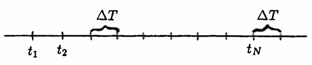
$P = N\Delta T = t_N - t_1 + \Delta T$
Any value of $\,K\,$ that is less than or equal to $\,\frac{N-1}2\,$ will meet the requirements of Theorems $1$ and $\,2\,.$ In the next definition, $\,K\,$ is usually taken to be as large as possible, subject to the condition $\,K\le\frac{N-1}2\,.$
Let $\,N\,$ be a positive integer, and let $\,\{(t_i,y_i)\}_{i=1}^N\,$ be a data set with a time list $\,(t_1,\ldots,t_N)\,$ that is uniform with positive increment $\,\Delta T\,.$ Define $\,P := N\Delta T\,.$ Let $\,K\,$ be any positive integer less than or equal to $\,\frac{N-1}2\,.$
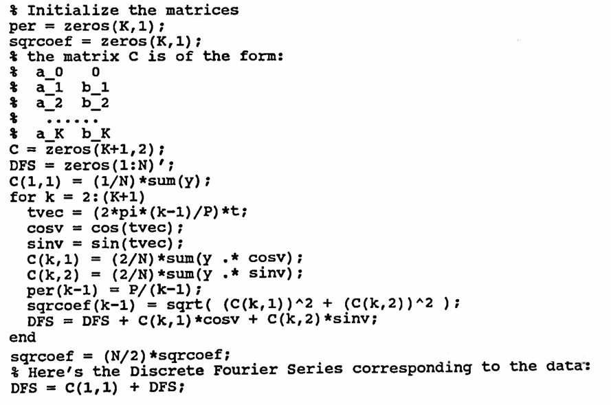
The discrete Fourier series corresponding to the data set and the chosen value $\,K\,$ is the function DFS given by
$$ \text{DFS}(t) := a_0 + \sum_{k=1}^K \bigl( a_k\cos\frac{2\pi kt}P + b_k\sin\frac{2\pi kt}P \bigr) \ , $$where the coefficients $\,a_0,a_1,\ldots,a_K,b_1,\ldots,b_K\,$ are given by:
$$ \begin{align} a_0 &= \frac 1N\sum_{n=1}^N y_n\ ,\cr\cr a_k &= \frac 2N\sum_{n=1}^N y_n\cos\frac{2\pi kt_n}P\ ,\ \ k = 1,\ldots,K\ ,\ \ \text{and}\cr\cr b_k &= \frac 2N\sum_{n=1}^N y_n\sin\frac{2\pi kt_n}P\ ,\ \ k = 1,\ldots,K \end{align} $$The graph of the points
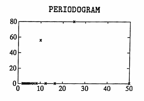
$$ \left\{ \left( \frac Pk\,,\, \frac N2\sqrt{a_k^2 + b_k^2} \right) \ |\ k = 1\ldots,K \right\} $$is the periodogram corresponding to the discrete Fourier series.
The reason for the factor $\,\frac N2\,$ in the definition of the periodogram will become apparent in the next section, on the discrete Fourier transform.
The periods of the sinusoids appearing in the discrete Fourier series are
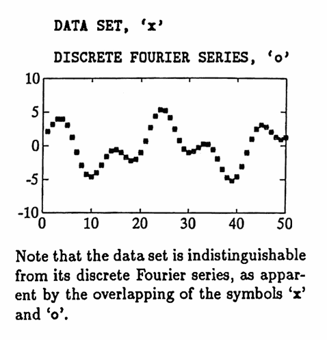
$$ P,\, \frac P2,\, \frac P3,\, \ldots,\,\frac PK\ ; $$the coefficients $\,a_k\,$ and $\,b_k\,$ multiply the sinusoids with period $\,\frac Pk\,.$ The coefficient $\,a_0\,$ gives the average of the data values. If $\,N = 2K + 1\,,$ then the discrete Fourier series passes through all the data points; and if $\,N \gt 2K + 1\,,$ then the series minimizes the mean-square error.
The periodogram gives information about ‘how much’ of each period is present in the data set, as the examples later on in this section will illustrate.
Observe that if one takes the formula for the continuous Fourier series coefficient $\,a_k\,,$
$$ a_k = \frac 2P\int_0^P g(t)\cos\frac{2\pi kt}P\,dt\ , $$replaces the $\,\int_0^P\,$ by $\,\sum_{n=1}^N\,,$ $\,dt\,$ by the increment $\,\frac PN\,,$ $\,t\,$ by $\,t_n\,,$ and $\,g(t)\,$ by $\,y_n\,,$ one obtains
$$ \begin{align} a_k &= \frac 2P\sum_{n=1}^N y_n \left( \cos\frac{2\pi kt_n}P \right) \cdot \frac PN\cr\cr &= \frac 2N\sum_{n=1}^N y_n\cos\frac{2\pi kt_n}P\ , \end{align} $$which is precisely the discrete Fourier coefficient $\,a_k\,.$ So there is a beautiful (and not unexpected) analogy between the continuous and discrete results.
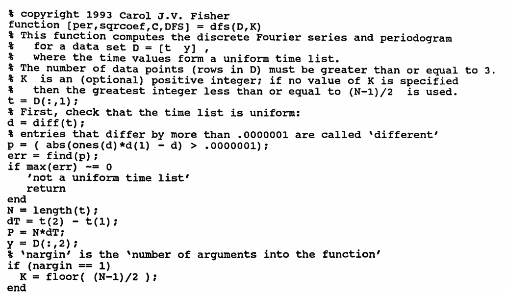
MATLAB Implementation: Discrete Fourier Series and the Periodogram
dfs(D,K)
The following MATLAB function computes the discrete Fourier
series and periodogram corresponding to a data set. To use the
program, type:
[per,sqrcoef,C,DFS] = dfs(D,K);
The required input is a data set $\,\{(t_i,y_i)\}_{i=1}^N\,,$ with $\, N \ge 3\,.$ The time values must be stored in a column vector t and the corresponding data values in a column vector y . Then, D = [t y] is the $\,N \times 2\,$ matrix containing the data set.
The time list contained in t must be uniform (increment $\,\Delta T \gt 0\,$). The program begins by checking that this requirement is met; if not, the program is halted and the message ‘not a uniform time list’ is displayed. (As written, increments between time values are said to ‘differ’ if they differ by more than $\,0.0000001\,.$ This value may be changed for different tolerances.)
The number $\,K\,$ must satisfy $\,N \ge 2K +1\,,$ that is, $\,K \le \frac{N-1}2\,.$ If no value of $\,K\,$ is supplied, then the program uses the greatest possible $\,K\,$ satisfying the stated requirement.
The output per is a column vector containing the periods $\,P,\,\frac P2,\,\frac P3,\,\ldots,\,\frac PK\,,$ where $\,P = N\Delta T\,.$
The output sqrcoef (for ‘square root ... coefficients’) is a column vector containing the numbers $\,\frac N2\sqrt{a_k^2 + b_k^2}\,$ for $\,k = 1,\ldots,K\,.$
The periodogram is then obtained with the command:
plot(per,sqrcoef)
If only the outputs
per
and
sqrcoef
are desired, the shorter command
[per,sqrcoef] = dfs(D);
or
[per,sqrcoef] = dfs(D,K);
may be used.
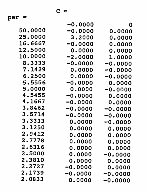
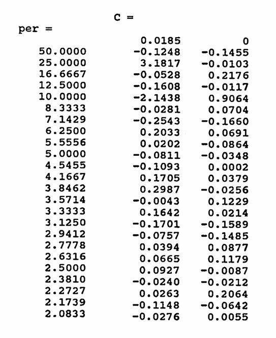
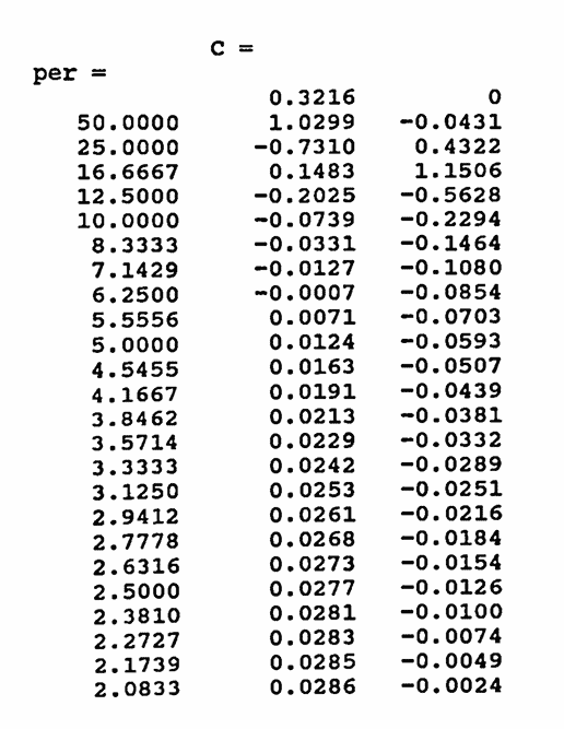
The (optional) output C is a column vector containing the coefficients $\,a_0,a_1,b_1,a_2,b_2,\ldots,a_K,b_K\,$ (in the order given).
The (optional) output DFS is a column vector containing the values $\,\text{DFS}(t_n)\,$ for $\,n = 1,\ldots, N\,.$
The source code for the function dfs is given next.
OCTAVE requires three changes:
-
You must write
ones(size(d))
instead of
ones(d) -
You must write
DFS = zeros(1,N)';
instead of
DFS = zeros(1:N)'; -
The last line of the function must be:
endfunction
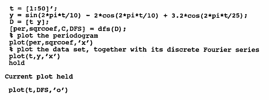
MATLAB Example: Sinusoidal Components, Periods in the DFS
In this first example, a data set is constructed having sinusoidal components of periods $\,25\,$ and $\,10\,.$ Fifty data points are used, with $\,\Delta T = 1\,,$ so that $\,P = (50)(1) = 50\,.$ The largest allowable value of $\,K\,$ is used: since $\,K \le \frac{50-1}2\,,$ the greatest such $\,K\,$ equals $\,24\,.$ Observe that the periods $\,\frac P5 = 10\,$ and $\,\frac P2 = 25\,$ appear in the discrete Fourier series.
First, the ‘pure’ data (no noise) is analyzed. Of course, the discrete Fourier series ‘recovers’ the components perfectly in this case.
Then, some noise is added to the data. In this case, the periodogram clearly peaks at periods $\,10\,$ and $\,25\,.$ However, the noise has contributed some small amplitude, high frequency (small period) components in the discrete Fourier series.
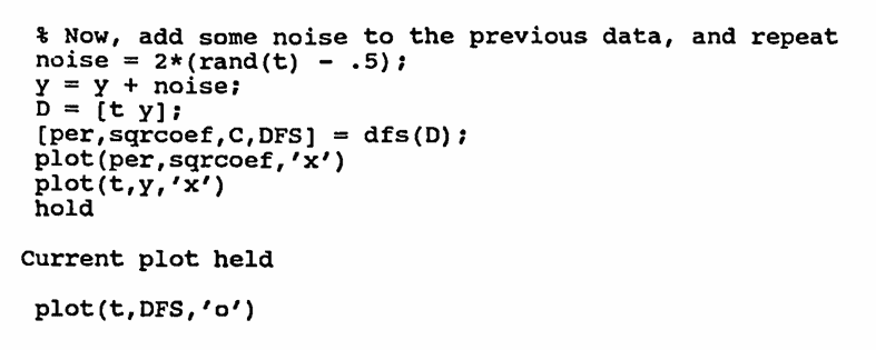
noise = 2*(rand(size(t)) - .5);
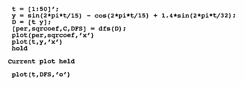
MATLAB Example: Sinusoidal Components, Periods are not in the DFS
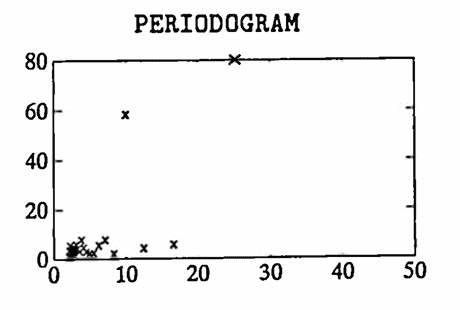
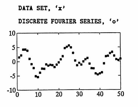
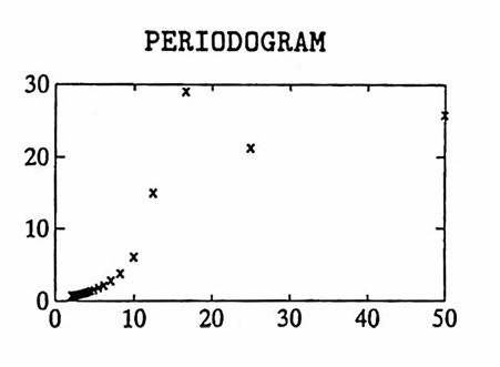
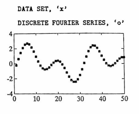
In this second example, a data set is constructed having sinusoidal components of periods $\,15\,$ and $\,32\,.$ Fifty data points are used, with $\,\Delta T = 1\,,$ so that again $\,P = (50)(1) = 50\,.$ Again, the largest allowable value of $\,K\,$ is used; $\,K = 24\,.$ Observe that the periods of the sinusoids in the data are not in the discrete Fourier series.
First, the ‘pure’ data (no noise) is analyzed. The periodogram ‘peaks’ at the period $\,\frac{50}3 = 16\frac 23\,,$ which is close to one of the ‘hidden’ periods, $\,15\,.$ The period $\,32\,$ component is not easily detectable from the periodogram.
Then, some noise is added to the data. The situation is similar to that described above, but with a little more ‘fuzz’.
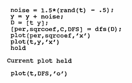
noise = 1.5*(rand(size(t)) - .5);
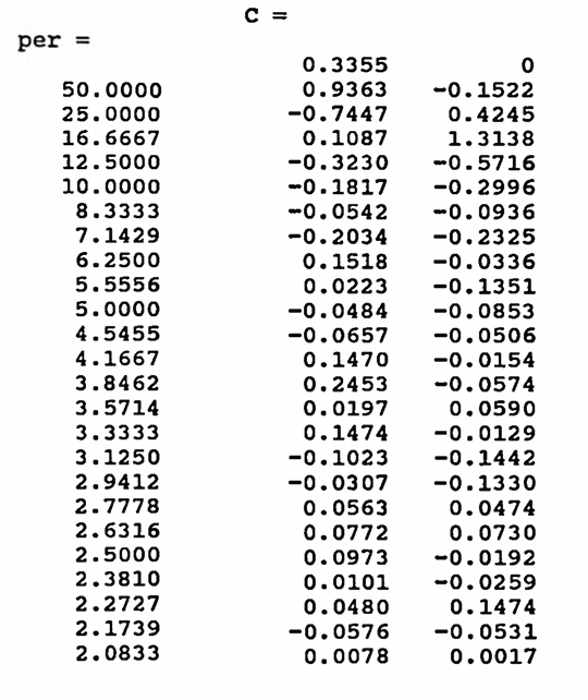
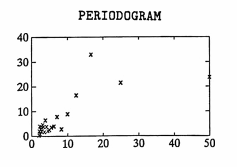
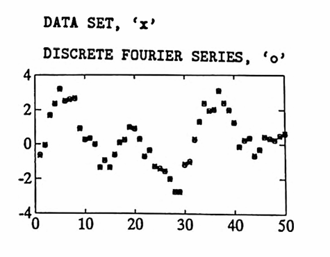
MATLAB Example: Periodogram of Noise
‘Noise’ is usually associated with high frequency (small period) components. In this example, the periodogram corresponding to some noise (from a uniform distribution) is found:
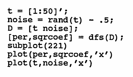
noise = rand(size(t)) - .5;
subplot(221) is optional (if you want smaller plots).
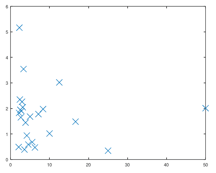
Periodogram
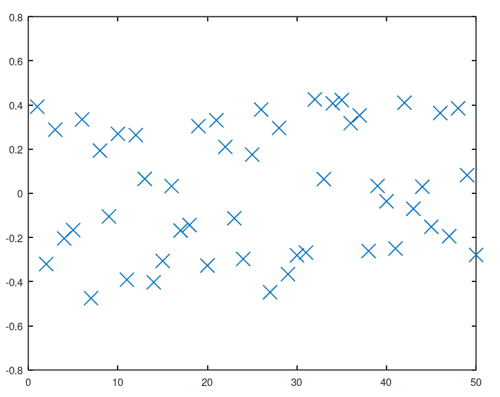
Data Set
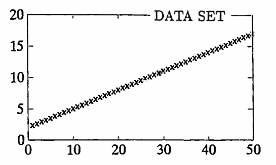
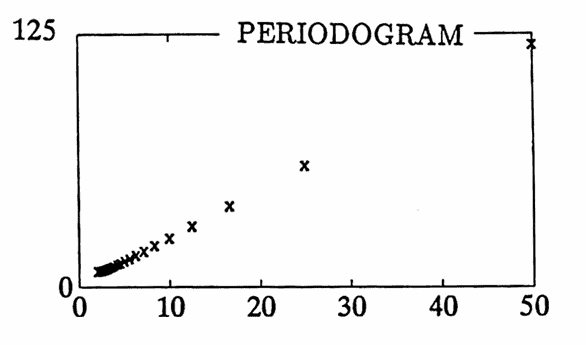
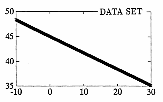
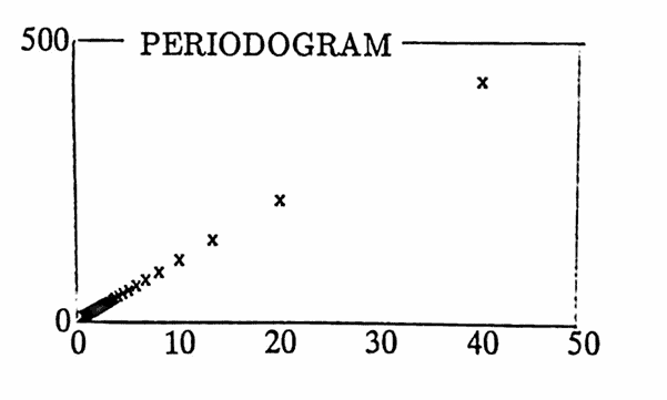
MATLAB Example: Periodogram of a ‘Ramp’
The periodograms of a couple ‘ramps’ (linear functions) are found next:
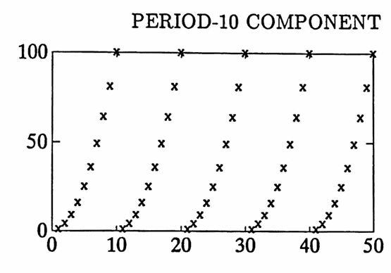
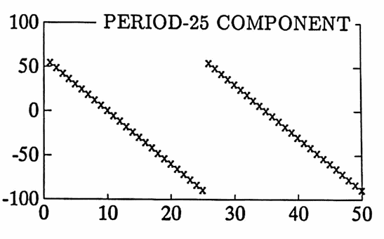
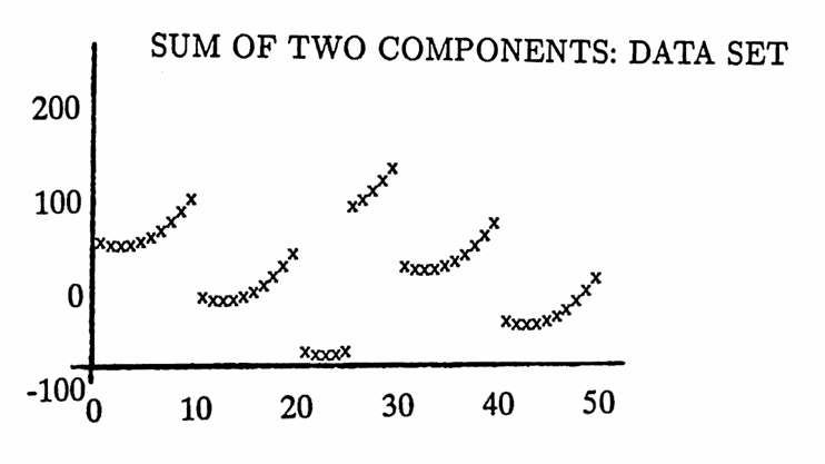
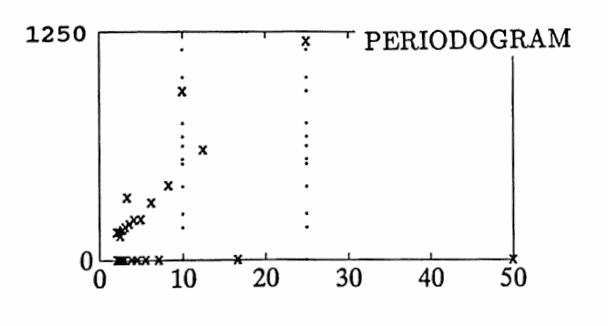
MATLAB Example: Non-Sinusoidal Components
Finally, the periodogram of a data set with two non-sinusoidal components, periods $\,10\,$ and $\,25\,,$ are found. Here, $\,N\Delta T = (50)(1)\,,$ so these periods $\,\frac{50}5 = 10\,$ and $\,\frac{50}2 = 25\,$ appear in the discrete Fourier series.
The vertical ‘dotted’ lines on the periodogram indicate the periods $\,10\,$ and $\,25\,.$ Observe that the periodogram does appear to ‘peak’ at these values.