An equation in two variables (like $\,y = x^2\,$) describes a set of points in the plane—the set of points
$\,(x,y)\,$ that make the equation true.
However, it's a static collection of points,
with no concept of the curve being ‘swept out’ (traced/drawn) in any particular way.
Parametric equations describe a
curve that is swept out in a particular way!
To illustrate:
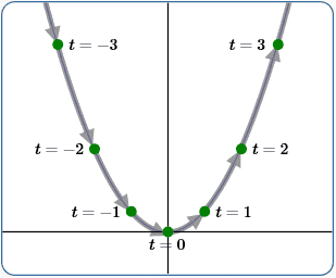
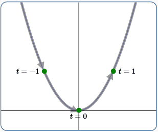
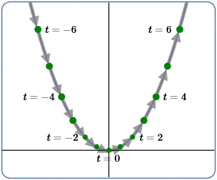
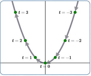
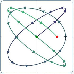
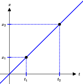
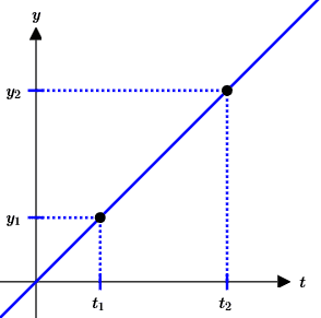
The four graphs below have precisely the same set of points, but are swept out in different ways.
Measure time $\,t\,$ in (say) seconds.
Then, each arrow below (connecting green points) represents a part of the curve traced out in one second.
|
|
|
|
|
(1) $x(t) = t\,$ $\,y(t) = t^2$ |
(2) $x(t) = 2t\,$ $\,y(t) = (2t)^2 = 4t^2$ |
(3) $x(t) = \frac 12t\,$ $\,y(t) = (\frac 12t)^2 = \frac{t^2}4$ |
(4) $x(t) = -t\,$ $\,y(t) = (-t)^2 = t^2$ |
| swept out from left to right |
swept from left to right, faster than in (1) |
swept from left to right, slower than in (1) |
swept from right to left, same speed as in (1) |
|
(Note:
For better-sized images, the horizontal and vertical scales on each individual graph are different. However, all four graphs use precisely the same scales.) |
|||
What is a parameter?
A parameter is a variable used
in a special way:
to identify particular members of a family of mathematical objects.
For example, consider the familiar equation $\,y = mx + b\,$.
Four variables appear in this equation ($\,x\,,$ $\,y\,,$ $\,m\,$ and $\,b\,$),
but only two of them ($\,m\,$ and $\,b\,$) are parameters.
Why?
The single equation ‘$\,y = mx + b\,$’ defines an entire family of equations.
Choices for $\,m\,$ and $\,b\,$ determine which member of this ‘family’ you get!
For example:
| choosing these parameters ... | ... gives this equation |
| $\,m = 2\,,$ $\,b = -1$ | $\,y = 2x - 1\,$ |
| $\,m = -3\,,$ $\,b = 0$ | $\,y = -3x\,$ |
| $\,m = 0\,,$ $\,b = 7\,$ | $\,y = 7\,$ |
| The list goes on and on! | |
As you'll learn below, parametric equations define a family of points instead of a family of equations, but the foundational idea is the same.
What are parametric equations?
Describe a curve in the following way:
-
Choose a parameter.
The variable $\,t\,$ is a common parameter choice, since it is often viewed as time. -
Give formulas, as functions of $\,t\,,$ for both the $x$-values and $y$-values of points on the curve.
That is (using function notation) write: $$ \cssId{s54}{ \begin{alignat}{2} x(t) &= \text{some function of $\,t\,$}&\qquad&\text{(read aloud as: ‘$\,x\,$ of $\,t\,$ is some function of $\,t\,$’)}\cr y(t) &= \text{some function of $\,t\,$}&\qquad&\text{(read aloud as: ‘$\,y\,$ of $\,t\,$ is some function of $\,t\,$’)}\cr \end{alignat}} $$
Together, these parametric equations describe a curve in a plane that is swept out in a particular way.
What is ‘parametric’ about parametric equations?
When a curve is described by parametric equations, you naturally get a family of points:
$$
\cssId{s59}{\text{all points of the form } \bigl(\,x(t)\,,\,y(t)\,\bigr) \text{ for the allowable values of $\,t\,$}}
$$
The parameter $\,t\,$ is used to identify each particular point in this family!
Note:
- In the ‘$\,y = mx + b\,$’ example, $\,m\,$ and $\,b\,$ are parameters to identify members in a family of equations.
- Parametric equations use a parameter (denoted here by $\,t\,$) to identify members in a family of points.
Some Interesting Parametric Equations
Here are some parametric equations that are more interesting than the simple examples at the top of this page.
Arrows and gradually-changing color have been added, so you can see how the curve is traced out.
Curves (except for Einstein) begin at the green point, and end at the red point.
For a given image, each arrow represents a part of the curve traced out in a fixed amount of time—so longer arrows means that piece is traced out faster!
The first three examples have additional parameters (other than $\,t\,$), so each describes an entire family of curves.
 (5) play with Lissajous curves $x(t) = A\sin(at + \delta)$ $y(t) = B\sin(bt)$ Here: $\,a = 5\,,$ $\,b = A = B = 4\,,$ $\,\delta = 0\,$ $\,t\in [0,\frac{5\pi}4]$ Note: it slows down going around curves |
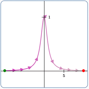 (6) Witch of Agnesi $x(t) = at$ $\displaystyle y(t) = a/(1+ t^2)$ Here: $\,a = 1$ $\,t\in [-10,10]$ |
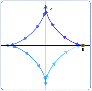 (7) Astroid $x(t) = a\,\cos^3 t$ $y(t) = a\,\sin^3 t$ Here: $\,a = 5\,$ $\,t\in [0,2\pi]$ (start and end points are the same) |
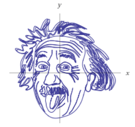 (8) an Albert Einstein curve After the linked page fully loads, scroll down to look at the equations for $\,x(t)\,$ and $\,y(t)\,.$ Pretty impressive! |
Notes about Parametric Equations
- A curve that is generated by parametric equations is called a parametric curve.
- Parametric equations can describe curves in space (as opposed to in a plane), by adding a third coordinate: $$\cssId{s102}{x = x(t)\,,\ \ \ y = y(t)\,,\ \ z = z(t)}$$
-
The equation $\,y = mx + b\,$ is an equation that uses parameters,
but it's not a parametric equation.
The phrase ‘parametric equation’ is typically reserved for situations where coordinates of points are described using parameter(s). - Bézier curves—important in computer graphics and animation (among other things)—are parametric curves.
Constructing a Parametric Curve with Desired Properties
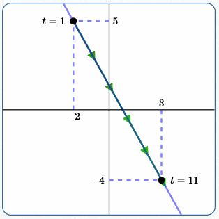
Suppose we want to travel between two fixed points, $\,P_1(x_1,y_1)\,$ and $\,P_2(x_2,y_2)\,,$ in a fixed time.
More specifically, we want to be at $\,P_1\,$ at time $\,t_1\,,$ and at $\,P_2\,$ at time $\,t_2\,$ (with $\,t_1\ne t_2\,$).
Of course, there are many different ways to travel between two points!
The simplest solution is a straight line path between the two.
Using function notation, we want:
|
$$ \begin{align} \cssId{s113}{x(t_1) = x_1}\cr \cssId{s114}{x(t_2) = x_2}\cr \cssId{s115}{y(t_1) = y_1}\cr \cssId{s116}{y(t_2) = y_2} \end{align} $$ |
|
Using point-slope form
in the $\,tx\,$-plane, we get:
$$
\begin{gather}
\cssId{s118}{x(t) - x_1 = \frac{x_2-x_1}{t_2-t_1}(t - t_1)}\cr\cr
\cssId{s119}{x(t) = x_1 + \frac{x_2-x_1}{t_2-t_1}(t - t_1)}\tag{9a}
\end{gather}
$$
Similarly,
$$
\cssId{s121}{y(t) = y_1 + \frac{y_2-y_1}{t_2-t_1}(t - t_1)}\tag{9b}
$$
Equations (9a) and (9b) are the desired parametric equations.
Together, they give a line through points $\,P_1(x_1,y_1)\,$ and $\,P_2(x_2,y_2)\,$ satisfying:
- at time $\,t_1\,$ you're at $\,P_1\,$
- at time $\,t_2\,$ you're at $\,P_2\,$
|
EXAMPLE: The line at right is at
|
 |
Eliminating the Parameter:
Going from a Parametric Curve to $\,y = f(x)\,$ (when possible)
Suppose a parametric curve passes a
vertical line test:
like examples 1, 2, 3, 4, 6, 9ab (but not 5, 7, 8).
Then, you may be able to get a description of the curve in the form ‘$\,y = f(x)\,$’.
In the ‘$\,y = f(x)\,$’ form, you lose information about how the curve is traced out,
but this single-equation form may be easier to work with for some applications.
When we want to emphasize that an $x$-value depends on (say) $\,t\,,$ we can write ‘$\,x = x(t)\,$’.
Read this aloud as: ‘$\,x\,$ equals $\,x\,$ of $\,t\,$’, meaning that the $x$-value is a function of $\,t\,.$
In going from a pair of parametric equations ‘$\,x = x(t)\,$ and $\,y = y(t)\,$’ to a single equation ‘$\,y = f(x)\,$’,
the parameter $\,t\,$ has been eliminated—it is gone!
Therefore, this process is typically referred to as ‘eliminating the parameter’.
The process of eliminating the parameter is often used to help identify the graph of parametric equations.
It may be easier to recognize a curve in ‘$\,y = f(x)\,$’ form than in parametric equation form.
Example: Eliminating the Parameter in Examples 1–4
Procedure:
- drop function notation: that is, write $\,x(t)\,$ as simply $\,x\,$; write $\,y(t)\,$ as simply $\,y\,$
- solve for $\,t\,$ in a simplest equation; substitute this expression for $\,t\,$ into the remaining equation
Note:
- in examples 1–4, the equation for $\,x(t)\,$ is simplest to solve for $\,t\,$
- upon eliminating the parameter, all four curves give $\,y = x^2\,$
| (1) $$ \begin{alignat}{2} \cssId{s161}{x(t) = t\,,\ \ y(t) = t^2}&\qquad&&\cssId{s162}{\text{original parametric equations}}\cr\cr \cssId{s163}{x = t\,,\ \ y = t^2} &&&\cssId{s164}{\text{drop function notation}}\cr\cr \cssId{s165}{t = x}&&&\cssId{s166}{\text{solve for $\,t\,$ in simplest equation}}\cr\cr \cssId{s167}{y = t^2 = x^2}&&&\cssId{s168}{\text{substitute into remaining equation}}\cr\cr \cssId{s169}{y = x^2}&&&\cssId{s170}{\text{$\,y = f(x)\,$ form}} \end{alignat} $$ | (2) $$ \begin{alignat}{2} \cssId{s172}{x(t) = 2t\,,\ \ y(t) = 4t^2}&\qquad&&\cssId{s173}{\text{original parametric equations}}\cr\cr \cssId{s174}{x = 2t\,,\ \ y = 4t^2} &&&\cssId{s175}{\text{drop function notation}}\cr\cr \cssId{s176}{t = \frac x2}&&&\cssId{s177}{\text{solve for $\,t\,$ in simplest equation}}\cr\cr \cssId{s178}{y = 4t^2 = 4\bigl(\frac x2\bigl)^2 = \frac{4x^2}{4} = x^2}&&&\cssId{s179}{\text{substitute into remaining equation}}\cr\cr \cssId{s180}{y = x^2}&&&\cssId{s181}{\text{$\,y = f(x)\,$ form}} \end{alignat} $$ |
| (3) $$ \begin{alignat}{2} \cssId{s183}{x(t) = \frac 12t\,,\ \ y(t) = \frac{t^2}4}&\qquad&&\cssId{s184}{\text{original parametric equations}}\cr\cr \cssId{s185}{x = \frac 12t\,,\ \ y = \frac{t^2}4} &&&\cssId{s186}{\text{drop function notation}}\cr\cr \cssId{s187}{t = 2x}&&&\cssId{s188}{\text{solve for $\,t\,$ in simplest equation}}\cr\cr \cssId{s189}{y = \frac{t^2}4 = \frac{(2x)^2}4 = \frac{4x^2}4 = x^2}&&&\cssId{s190}{\text{substitute into remaining equation}}\cr\cr \cssId{s191}{y = x^2}&&&\cssId{s192}{\text{$\,y = f(x)\,$ form}} \end{alignat} $$ | (4) $$ \begin{alignat}{2} \cssId{s194}{x(t) = -t\,,\ \ y(t) = t^2}&\qquad&&\cssId{s195}{\text{original parametric equations}}\cr\cr \cssId{s196}{x = -t\,,\ \ y = t^2} &&&\cssId{s197}{\text{drop function notation}}\cr\cr \cssId{s198}{t = -x}&&&\cssId{s199}{\text{solve for $\,t\,$ in simplest equation}}\cr\cr \cssId{s200}{y = t^2 = (-x)^2 = x^2}&&&\cssId{s201}{\text{substitute into remaining equation}}\cr\cr \cssId{s202}{y = x^2}&&&\cssId{s203}{\text{$\,y = f(x)\,$ form}} \end{alignat} $$ |
Example: Eliminating the Parameter in 9ab
To eliminate the parameter, you don't have to solve for (just) $\,t\,.$
As illustrated in this example,
it's sometimes easier to solve for a different expression (involving $\,t\,$) that appears in both $\,x(t)\,$ and $\,y(t)\,.$
Here, we solve for $\,t - t_1\,$:
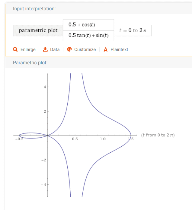
Parametric Equations at WolframAlpha
|
Hop up to WolframAlpha and type in (say): (You can cut-and-paste.) Voila! How easy is that? |
|
by practicing the exercise at the bottom of this page.
Congratulations on finishing Precalculus!!
Next up—Calculus!